DALLE’s Rendering of Non-Convex Optimization
In Life We Are Always Optimizing.
~ Professor Benard Widrow (inventor of the LMS algorithm)
Hello Folks! As always, i hope everyone is safe. i also hope everyone had a wonderful holiday break with food, family, and friends.
The first SnakeByte of the new year involves a subject near and dear to my heart: Optimization.
The quote above was from a class in adaptive signal processing that i took at Stanford from Professor Benard Widrow where he talked about how almost everything is a gradient type of optimization and “In Life We Are Always Optimizing.”. Incredibly profound if One ponders the underlying meaning thereof.
So why optimization?
Well glad you asked Dear Reader. There are essentially two large buckets of optimization: Convex and Non Convex optimization.
Convex optimization is an optimization problem has a single optimal solution that is also the global optimal solution. Convex optimization problems are efficient and can be solved for huge issues. Examples of convex optimization include maximizing stock market portfolio returns, estimating machine learning model parameters, and minimizing power consumption in electronic circuits.
Non-convex optimization is an optimization problem can have multiple locally optimal points, and it can be challenging to determine if the problem has no solution or if the solution is global. Non-convex optimization problems can be more difficult to deal with than convex problems and can take a long time to solve. Optimization algorithms like gradient descent with random initialization and annealing can help find reasonable solutions for non-convex optimization problems.
You can determine if a function is convex by taking its second derivative. If the second derivative is greater than or equal to zero for all values of x in an interval, then the function is convex. Ah calculus 101 to the rescue.
Caveat Emptor, these are very broad mathematically defined brush strokes.
So why do you care?
Once again, Oh Dear Reader, glad you asked.
Non-convex optimization is fundamentally linked to how neural networks work, particularly in the training process, where the network learns from data by minimizing a loss function. Here’s how non-convex optimization connects to neural networks:
A loss function is a global function for convex optimization. A “loss landscape” in a neural network refers to representation across the entire parameter space or landscape, essentially depicting how the loss value changes as the network’s weights are adjusted, creating a multidimensional surface where low points represent areas with minimal loss and high points represent areas with high loss; it allows researchers to analyze the geometry of the loss function to understand the training process and potential challenges like local minima. To note the weights can be millions, billions or trillions. It’s the basis for the cognitive AI arms race, if you will.
The loss function in neural networks, measures the difference between predicted and true outputs, is often a highly complex, non-convex function. This is due to:
The multi-layered structure of neural networks, where each layer introduces non-linear transformations and the high dimensionality of the parameter space, as networks can have millions, billions or trillions of parameters (weights and biases vectors).
As a result, the optimization process involves navigating a rugged loss landscape with multiple local minima, saddle points, and plateaus.
Optimization Algorithms in Non-Convex Settings
Training a neural network involves finding a set of parameters that minimize the loss function. This is typically done using optimization algorithms like gradient descent and its variants. While these algorithms are not guaranteed to find the global minimum in a non-convex landscape, they aim to reach a point where the loss is sufficiently low for practical purposes.
This leads to the latest SnakeBtye[18]. The process of optimizing these parameters is often called hyperparameter optimization. Also, relative to this process, designing things like aircraft wings, warehouses, and the like is called Multi-Objective Optimization, where you have multiple optimization points.
As always, there are test cases. In this case, you can test your optimization algorithm on a function called The Himmelblau’s function. The Himmelblau Function was introduced by David Himmelblau in 1972 and is a mathematical benchmark function used to test the performance and robustness of optimization algorithms. It is defined as:
![]()
Using Wolfram Mathematica to visualize this function (as i didn’t know what it looked like…) relative to solving for ![]() :
:

Wolfram Plot Of The Himmelblau Function
This function is particularly significant in optimization and machine learning due to its unique landscape, which includes four global minima located at distinct points. These minima create a challenging environment for optimization algorithms, especially when dealing with non-linear, non-convex search spaces. Get the connection to large-scale neural networks? (aka Deep Learnin…)
The Himmelblau’s function is continuous and differentiable, making it suitable for gradient-based methods while still being complex enough to test heuristic approaches like genetic algorithms, particle swarm optimization, and simulated annealing. The function’s four minima demand algorithms to effectively explore and exploit the gradient search space, ensuring that solutions are not prematurely trapped in local optima.
Researchers use it to evaluate how well an algorithm navigates a multi-modal surface, balancing exploration (global search) with exploitation (local refinement). Its widespread adoption has made it a standard in algorithm development and performance assessment.
Several types of libraries exist to perform Multi-Objective or Parameter Optimization. This blog concerns one that is extremely flexible, called OpenMDAO.
What Does OpenMDAO Accomplish, and Why Is It Important?
OpenMDAO (Open-source Multidisciplinary Design Analysis and Optimization) is an open-source framework developed by NASA to facilitate multidisciplinary design, analysis, and optimization (MDAO). It provides tools for integrating various disciplines into a cohesive computational framework, enabling the design and optimization of complex engineering systems.
Key Features of OpenMDAO Integration:
OpenMDAO allows engineers and researchers to couple different models into a unified computational graph, such as aerodynamics, structures, propulsion, thermal systems, and hyperparameter machine learning. This integration is crucial for studying interactions and trade-offs between disciplines.
Automatic Differentiation:
A standout feature of OpenMDAO is its support for automatic differentiation, which provides accurate gradients for optimization. These gradients are essential for efficient gradient-based optimization techniques, particularly in high-dimensional design spaces. Ah that calculus 101 stuff again.
It supports various optimization methods, including gradient-based and heuristic approaches, allowing it to handle linear and non-linear problems effectively.
By making advanced optimization techniques accessible, OpenMDAO facilitates cutting-edge research in system design and pushes the boundaries of what is achievable in engineering.
Lo and Behold! OpenMDAO itself is a Python library! It is written in Python and designed for use within the Python programming environment. This allows users to leverage Python’s extensive ecosystem of libraries while building and solving multidisciplinary optimization problems.
So i had the idea to use and test OpenMDAO on The Himmelblau function. You might as well test an industry-standard library on an industry-standard function!
First things first, pip install or anaconda:
>> pip install 'openmdao[all]'Next, being We are going to be plotting stuff within JupyterLab i always forget to enable it with the majik command:
## main code
%matplotlib inline
Ok lets get to the good stuff the code.
# add your imports here:
import numpy as np
import matplotlib.pyplot as plt
from openmdao.api import Problem, IndepVarComp, ExecComp, ScipyOptimizeDriver
# NOTE: the scipy import

# Define the OpenMDAO optimization problem - almost like self.self
prob = Problem()

# Add independent variables x and y and make a guess of X and Y:
indeps = prob.model.add_subsystem('indeps', IndepVarComp(), promotes_outputs=['*'])
indeps.add_output('x', val=0.0)  # Initial guess for x
indeps.add_output('y', val=0.0)  # Initial guess for y

# Add the Himmelblau objective function. See the equation from the Wolfram Plot?
prob.model.add_subsystem('obj_comp', ExecComp('f = (x**2 + y - 11)**2 + (x + y**2 - 7)**2'), promotes_inputs=['x', 'y'], promotes_outputs=['f'])

# Specify the optimization driver and eplison error bounbs.  ScipyOptimizeDriver wraps the optimizers in *scipy.optimize.minimize*. In this example, we use the SLSQP optimizer to find the minimum of the "Paraboloid" type optimization:
prob.driver = ScipyOptimizeDriver()
prob.driver.options['optimizer'] = 'SLSQP'
prob.driver.options['tol'] = 1e-6

# Set design variables and bounds
prob.model.add_design_var('x', lower=-10, upper=10)
prob.model.add_design_var('y', lower=-10, upper=10)

# Add the objective function Himmelblau via promotes.output['f']:
prob.model.add_objective('f')

# Setup and run the problem and cross your fingers:
prob.setup()
prob.run_driver()
Dear Reader, You should see something like this:
Optimization terminated successfully (Exit mode 0)
Current function value: 9.495162792777827e-11
Iterations: 10
Function evaluations: 14
Gradient evaluations: 10
Optimization Complete
———————————–
Optimal x: [3.0000008]
Optimal y: [1.99999743]
Optimal f(x, y): [9.49516279e-11]
So this optimized the minima of the function relative to the bounds of ![]() and
and ![]() and
and ![]() .
.
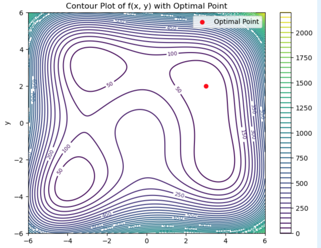
Now, lets look at the cool eye candy in several ways:
# Retrieve the optimized values
x_opt = prob['x']
y_opt = prob['y']
f_opt = prob['f']

print(f"Optimal x: {x_opt}")
print(f"Optimal y: {y_opt}")
print(f"Optimal f(x, y): {f_opt}")

# Plot the function and optimal point
x = np.linspace(-6, 6, 400)
y = np.linspace(-6, 6, 400)
X, Y = np.meshgrid(x, y)
Z = (X**2 + Y - 11)**2 + (X + Y**2 - 7)**2

plt.figure(figsize=(8, 6))
contour = plt.contour(X, Y, Z, levels=50, cmap='viridis')
plt.clabel(contour, inline=True, fontsize=8)
plt.scatter(x_opt, y_opt, color='red', label='Optimal Point')
plt.title("Contour Plot of f(x, y) with Optimal Point")
plt.xlabel("x")
plt.ylabel("y")
plt.legend()
plt.colorbar(contour)
plt.show()
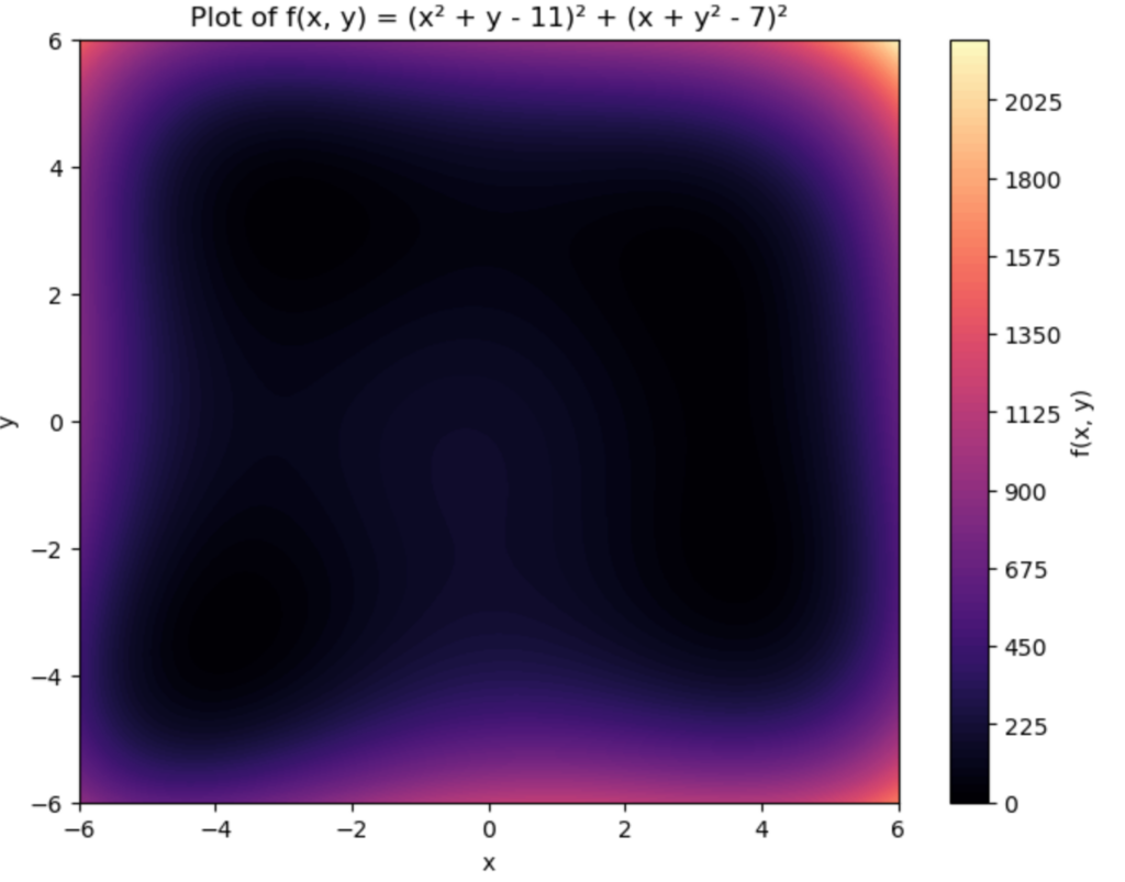
Now, lets try something that looks a little more exciting:
import numpy as np
import matplotlib.pyplot as plt

# Define the function
def f(x, y):
    return (x**2 + y - 11)**2 + (x + y**2 - 7)**2

# Generate a grid of x and y values
x = np.linspace(-6, 6, 500)
y = np.linspace(-6, 6, 500)
X, Y = np.meshgrid(x, y)
Z = f(X, Y)

# Plot the function
plt.figure(figsize=(8, 6))
plt.contourf(X, Y, Z, levels=100, cmap='magma')  # Gradient color
plt.colorbar(label='f(x, y)')
plt.title("Plot of f(x, y) = (x² + y - 11)² + (x + y² - 7)²")
plt.xlabel("x")
plt.ylabel("y")
plt.show()

That is cool looking.
Ok, lets take this even further:
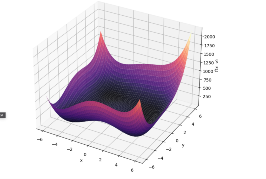
We can compare it to the Wolfram Function 3D plot:
from mpl_toolkits.mplot3d import Axes3D

# Create a 3D plot
fig = plt.figure(figsize=(10, 8))
ax = fig.add_subplot(111, projection='3d')

# Plot the surface
ax.plot_surface(X, Y, Z, cmap='magma', edgecolor='none', alpha=0.9)

# Labels and title
ax.set_title("3D Plot of f(x, y) = (x² + y - 11)² + (x + y² - 7)²")
ax.set_xlabel("x")
ax.set_ylabel("y")
ax.set_zlabel("f(x, y)")

plt.show()
Which gives you a 3D plot of the function:

3D Plot of f(x, y) = (x² + y – 11)² + (x + y² – 7)²
While this was a toy example for OpenMDAO, it is also a critical tool for advancing multidisciplinary optimization in engineering. Its robust capabilities, open-source nature, and focus on efficient computation of derivatives make it invaluable for researchers and practitioners seeking to tackle the complexities of modern system design.
i hope you find it useful.
Until Then,
#iwishyouwater <- The EDDIE – the most famous big wave contest ran this year. i saw it on the beach in 2004 and got washed across e rivermouth on a 60ft clean up set that washed out the river.
Music To Blog By: GodSpeedYouBlackEmperor “No Title As of 13 February 2024” – great band if you enjoy atmospheric compositional music.
