Computational_Economics | Theodore C. Tanner Jr.

Pre-Computing War

Sora’s idea of a Neon Drone War With Audio Track

Sometimes it is the people no one can imagine anything of who do the things no one can imagine.

~ Alan Turing

First, i trust everyone is safe. Second, i had a creative spurt of late and wrote the following blog in one sitting after waking up thinking about the subject.

NOTE: This post is in no way indicative of any stance or provides any classified information whatsoever. It is only a thought piece concerning current technology-driven areas of concern.

Preamble

There is a paradigm shift happening that will affect future generations and possibly the very essence of what it means to be human, and this comes from how technology is transforming war. We stand at a precipice, gazing into a future where the tools of war no longer resemble the clashing steel and human courage of centuries past. How important is conflict to humanity? What is the essence and desire for this conflict? The current uptick in drone usage of the past years has created an inflection point for what I am terming “abstraction levels for engagement.”

We continue to underestimate how important drones are going to be in warfare—a miscalculation that echoes through history’s long ledger of missed signals. I’m going to go out on a long limb here and say the future of most warfare will be enabled by, driven by, and spearheaded by drones. In fact, other than some other types of autonomous vehicles, there might not be anything else on the battlefield.

Here is a definition (of course, AI bot generated because really who reads Webster’s Dictionary nowadays? For the record, i have read Webster’s 3 times front to back):

“A military drone, also known as an unmanned aerial vehicle (UAV) or unmanned aircraft system (UAS), is an aircraft flown without a human pilot on board, controlled remotely or autonomously, and used for military missions like surveillance, reconnaissance, and potentially combat operations. “

This isn’t hyperbole; it’s the logical endpoint of a trajectory we’ve been on since the first unmanned systems took flight. And at the end of that trajectory lies something even more radical: autonomous bullets—not merely guided, but self-directed, a fusion of machine intelligence and lethal intent that could redefine conflict itself.

Note: I edited this part as the kind folk on The LazyWeb(tm) were laser-focused on the how of “smart bullets.: Great feedback and thank you. git push -u -f origin main.

Guided autonomous bullets, often referred to as “smart bullets,” represent an advanced leap in projectile technology, blending precision guidance systems with small-caliber ammunition. These bullets are designed to adjust their flight path mid-air to hit a target with exceptional accuracy, even if the target is moving or environmental factors like wind interfere. The concept builds on precision guided munitions used in larger systems like missiles, but shrinks the technology to fit within the constraints of a bullet fired from a firearm.

Autonomous bullets, often referred to as “smart bullets,” are advanced projectiles designed to adjust their trajectory mid-flight to hit a target with high precision, even under challenging conditions like wind or a moving target. While the concept might sound like science fiction, significant research has been conducted, particularly by organizations like DARPA (Defense Advanced Research Projects Agency) and Sandia National Laboratories, to make this technology a reality.

The core idea behind autonomous bullets is to integrate guidance systems into small-caliber projectiles, allowing them to self-correct their path after being fired. One of the earliest designs, as described in “historical research”, involved a bullet with three fiber-optic sensors (or “eyes”) positioned around its circumference to provide three-dimensional awareness. A laser is used to designate the target, and as the bullet travels, these sensors detect the laser’s light. The bullet adjusts its flight path in real time to ensure an equal amount of laser light enters each sensor, effectively steering itself toward the laser-illuminated target. This method prevents the bullet from making drastic turns like a missile. Still, it enables small, precise adjustments to hit exactly where the laser is pointed, even if the target is beyond visual range or the laser source is separate from the shooter. It hath been said that if you can think it DARPA has probably built it, maybe.

Given the advancements in drones, unmanned autonomous vehicles, land and air vehicles, and supposedly smart bullets (only the dark web knows how they work), imagine a battlefield stripped of human presence, not out of cowardice but necessity. The skies a deafening hum with swarms of drones (if a drone makes a sound and no one is there to hear it, does it make a sound?), each a “node” orchestrated via particle swarm AI models in a vast, decentralized network of artificial minds.

No generals barking orders, no soldiers trudging through mud, just silicon and steel executing a dance of destruction with precision beyond human capacity. The end state of drones isn’t just remote control or pre-programmed strikes; it’s autonomy so complete that the machines themselves decide who lives and who dies – no human in the loop. Self-directed projectiles, bullets with brains roaming the theater of war, seeking targets based on algorithms fed by real-time data streams. The vision feels like science fiction, yet the pieces already fall into place.

Generals gathered in their masses
just like witches at black masses
evil minds that plot destruction
sorcerers of death’s construction
in the fields the bodies burning
as the war machine keeps turning
death and hatred to mankind
poisoning their brainwashed minds, oh lord yeah!

~ War Pigs, Black Sabbath 1970

This shift isn’t merely tactical; it’s existential. Warfare has always been a contest of wills, a brutal arithmetic of resources and resolve. But what happens when we can compute the outcome before the first shot is fired? Drones, paired with advanced AI, offer the tantalizing possibility of simulating conflicts down to the last variable terrain, weather, enemy morale, and supply lines, all processed in milliseconds by systems that learn as they go. The autonomous bullet isn’t just a weapon; it’s a data point in a larger Markovian equation, one that could predict victory or defeat with chilling accuracy.

We’re not far from a world where wars are fought first in the cloud, their outcomes modeled and refined, before a single drone lifts off.If the future of warfare is of drone swarms of autonomous systems culminating in self-directed bullets, then pre-computing its outcomes becomes not just feasible but imperative. The battlefield of tomorrow isn’t a chaotic melee; it’s a high-stakes game, a multidimensional orchestrated chessboard where game theory, geopolitics, and macroeconomics converge to predict the endgame before the first move. To compute warfare in this way requires us to distill its essence into variables, probabilities, and incentives a task as daunting as it is inevitable. Yet again, there exists a terminology for this orchestrated chess game. Autonomous asymmetric mosaic warfighting, a concept explored by DARPA, envisions turning complexity into an asymmetric advantage by using networked, smaller, and less complex systems to overwhelm an adversary with a multitude of capabilitiesnvisions turning complexity into an asymmetric advantage by using networked, smaller, and less complex systems to overwhelm an adversary with a multitude of capabilities.

“A Nash equilibrium is a set of strategies that players act out, with the property that no player benefits from changing their strategy. ~ Dr John Nash.”

Computational Game Theory: The Logic of Lethality

At its core, warfare is a strategic interaction, a contest where players, nations, factions, or even rogue actors vie for dominance under the constraints of resources and information. Game theory offers the scaffolding to model this. Imagine a scenario where drones dominate: each side deploys autonomous swarms, programmed with decision trees that weigh attack, retreat, or feint based on real-time data. The payoff matrix isn’t just about territory or casualties, it’s about disruption, deterrence, and psychological impact. A swarm’s choice to strike a supply line rather than a command center could shift an enemy’s strategy, forcing a cascade of recalculations.

Now, introduce autonomous bullets, self-directed agents within the swarm. Each bullet becomes a player in a sub-game, optimizing its path to maximize damage while minimizing exposure. The challenge lies in anticipating the opponent’s moves: if both sides rely on AI-driven systems, the game becomes a duel of algorithms, each trying to out-predict the other. Zero-sum models give way to dynamic equilibria, where outcomes hinge on how well each side’s AI can bluff, adapt, or exploit flaws in the other’s logic. Pre-computing this requires vast datasets, historical conflicts, behavioral patterns, and even cultural tendencies fed into simulations that run millions of iterations, spitting out probabilities of victory, stalemate, or collapse.

Geopolitics: The Board Beyond the Battlefield

Warfare doesn’t exist in a vacuum; the shifting tectonic plates of geopolitics shape it. To pre-compute outcomes, we must map the global chessboard—alliances, rivalries, and spheres of influence. Drones level the playing field, but their deployment reflects deeper asymmetries. A superpower with advanced AI and manufacturing might flood the skies with swarms, while a smaller state leans on guerrilla tactics, using cheap, hacked drones to harass and destabilize. The game-theoretic model expands: players aren’t just combatants but also suppliers, proxies, and neutral powers with their own agendas.

Take energy as a (the main) variable: drones require batteries, rare earths, and infrastructure. A nation controlling lithium mines or chip fabs holds leverage, tipping the simulation’s odds. Sanctions, trade routes, and cyber vulnerabilities—like a rival hacking your drone fleet’s firmware—become inputs in the equation. Geopolitical stability itself becomes a factor: if a war’s outcome hinges on a fragile ally, the model must account for the likelihood of defection or collapse. Pre-computing warfare here means forecasting not just the battle, but the ripple effects—will a decisive drone strike trigger a refugee crisis, a shift in NATO’s posture, or a scramble for Arctic resources? The algorithm must think in networks, not lines.

I visualize a time when we will be to robots what dogs are to humans, and I’m rooting for the machines.

~ Claude Shannon

Macroeconomics: The Sinews of Silicon War

No war is won without money, and drones don’t change that; they just rewrite the budget. Pre-computing conflict demands a macroeconomic lens: how much does it cost to field a swarm versus defend against one? The economics of autonomous warfare favor scale mass-produced drones and bullets could outpace legacy systems like jets or tanks in cost-efficiency. A simulation might pit a 10 billion dollar defense budget against a 1 billion dollar insurgent force, factoring in production rates, maintenance, and the price of countermeasures like EMPs or jamming tech.

But it’s not just about direct costs. Markets react to war’s shadow oil spikes, currencies wobble, tech stocks soar or crash based on who controls the drone supply chain (it is all about that theta/beta folks). A protracted conflict could drain a nation’s reserves, while a swift, computed victory might bolster its credit rating. The model must integrate these feedback loops: if a drone war craters a rival’s economy, their ability to replenish dwindles, tilting the odds. And what of the peacetime economy? States that mastering autonomous tech could dominate postwar reconstruction, turning military R&D into a geopolitical multiplier. Pre-computing this requires economic forecasts layered atop the game-theoretic core—GDP growth, inflation, and consumer confidence as resilience proxies.

The Supreme Lord said: I am mighty Time, the source of destruction that comes forth to annihilate the worlds. Even without your participation, the warriors arrayed in the opposing army shall cease to exist.~ Bhagavad Gita 11:32

The Synthesis: Simulating the Unthinkable

To tie it all together, picture a supercomputer or a distributed AI network running a grand simulation. It ingests game-theoretic strategies (strike patterns, bluffing probabilities), geopolitical alignments (alliances, resource choke points), and macroeconomic trends (war budgets, trade disruptions). Drones and their autonomous bullets are the pawns, but the players are human decision-makers, constrained by politics and profit. The system runs countless scenarios: a drone swarm cripples a port, triggering a naval response, spiking oil prices, and collapsing a coalition. Another sees a small state’s cheap drones hold off a giant, forcing a negotiated peace.

The output isn’t a single prediction, but a spectrum 75% chance of victory if X holds, 40% if Y defects, 10% if the economy tanks. Commanders could tweak inputs more drones, better AI, a preemptive cyberstrike and watch the probabilities shift. It’s not infallible; black swans like a rogue AI bug or a sudden uprising defy the math. But it’s close enough to turn war into a science, reducing the fog Clausewitz warned of to a manageable haze [1].

The thing that hath been, it is that which shall be; and that which is done is that which shall be done: and there is no new thing under the sun.

~ Ecclesiastes 1:9, KJV

Yet, this raises a haunting question: If we can compute warfare’s endgame, do we lose something essential in the process?

The chaos of flawed, emotional, unpredictable human decision-making has long been the wildcard that defies calculation. Napoleon’s audacity, the Blitz’s resilience, and the guerrilla fighters’ improvisation are not easily reduced to code. Drones and their self-directed progeny promise efficiency, but they also threaten to strip war of its human texture, turning it into a sterile exercise in optimization. And what of accountability? When a bullet chooses its target, who bears the moral weight—the coder, the commander, or the machine itself?

The implications stretch beyond the battlefield. If drones dominate warfare, the barriers to entry collapse. No longer will nations need vast armies or industrial might; a few clever engineers and a swarm of cheap, autonomous systems could level the playing field. We’ve seen glimpses of this in Ukraine, where off-the-shelf drones have humbled tanks and disrupted supply lines. Scale that up, and the future isn’t just drones it’s a proliferation of power, a democratization of destruction. Autonomous bullets could become the ultimate equalizer or the ultimate chaos agent, depending on who wields them.

Fighting for peace is like screwing for virginity.

~ George Carlin

A Moment of Clarity

i wonder: are we ready to surrender the reins? The dream of computing warfare’s outcome is seductive and humans are carnal creatures we lust for other humans and things, thus it promises to minimize loss, to replace guesswork with certainty, but it also risks turning us into spectators of our own fate, watching as machines play out scenarios we’ve set in motion (that which we lust after).

The end state of drones may indeed be a battlefield of self-directed systems, but the end state of humanity in that equation remains unclear. Perhaps the true revolution isn’t in the technology but in how we grapple with a world where war becomes a problem to be solved rather than a story to be lived.

We underestimate drones at our peril. They’re not just tools; they’re harbingers of a paradigm shift. The future is coming, and it’s buzzing overhead—relentless, autonomous, and utterly indifferent to our nostalgia for the wars of old.

Pre-computing warfare might make us too confident. Leaders who trust the model might rush to conflict, assuming the odds are locked. But humans aren’t algorithms; we rebel, err, and surprise. And what of ethics? A simulation that optimizes for victory might greenlight drone strikes on civilians to break morale, justified by a percentage point. The autonomous bullet doesn’t care; it’s our job to decide if the computation is worth the soul it costs.

In this drone-driven future, pre-computing warfare isn’t just possible—it’s already beginning. Ukraine’s drone labs, China’s swarm tests, the Pentagon’s AI budgets—they’re all steps toward a world where conflict is a solvable problem. It has been said that fighting and sex are the two book ends but one in the same. But as we build the machine to predict the fight, we must ask: are we mastering war, or merely handing it a new master for something else entirely?

Music To Blog By: Project-X “Closing Down The Systems. Actually, I wouldn’t listen to this if i were you, unless you want to have nightmares. Fearless (MZ412 Remix) does sound like computational warfare.

Until then,

#iwishyouwater <- recent raw Pipe footage of folks that got the memo.

Ted ℂ. Tanner Jr. (@tctjr) / X

References:

[1] “On War” by Carl von Clausewitz. He called it “The Fog of War”: Clausewitz stressed the importance of understanding the unpredictable nature of war, noting that the “fog of war” (i.e., incomplete, dubious, and often erroneous information and great fear, doubt, and excitement) can lead to rapid decisions by alert commanders.

[2] Thanks to Jay Sales for being the catalyst for this blog. If you do not know who he is look him up here. Jay Sales. One of the best engineering executives and dear friend.

NVIDIA GTC 2025: The Time Has Come The Valley Said

OpenAI’s idea of The Valley – Its Been A Minute

Embrace the unknown and embrace change. That’s where true breakthroughs happen.

~Jensen Huang

First i trust everyone is safe. Second i usually do not write about discrete events or “work” related items but this is an exception. March 17-21, 2025 i and some others attended NVIDIA GTC2025. It warranted a long writeup. Be Forewarned: tl;dr. Read on Dear Reader. Hope you enjoy this one as it is a sea change in computing and a tectonic ocean shift in technology.

NVIDIA GTC 2025: AI’s Raw Hot Buttered Future

March 17-21, 2025, San Jose became geek central for NVIDIA’s GTC—aka the “Super Bowl of AI.” Hybrid setup, in-person or virtual, didn’t matter; thousands of devs, researchers, and suits swarmed to see what’s cooking in AI, GPUs, and robotics. Jensen Huang dropped bombs in his keynote, 1,000+ sessions drilled into the guts of it, and big players flexed their wares. Here’s the raw dog buttered scoop—and why you should care if you sling code or ship product.

The time has come,’ the Walrus said,

      To talk of many things:

Of shoes — and ships — and sealing-wax —

      Of cabbages — and kings —

And why the sea is boiling hot —

      And whether pigs have wings.’

~ The Walrus and The Carpenter

All The Libraries

Jensen’s Keynote: AI’s Next Gear, No Hype

March 18, 2025 SAP Center and the MCenery Civic Center, over 28,000 geeks packed in both halls and out in the streets . Jensen Huang, NVIDIA’s leather-jacketed maestro, hit the stage and didn’t waste breath. 2.5 hours no notes and started with the top of the stack with all the libraries NVIDIA has “CUDA-ized” and went all the way down to the photonic ethernet cables. No corporate fluff, just tech meat for the developer carnivore. His pitch: AI’s not just chatbots anymore; it’s “agentic,” thinking and moving in the real world forward at the speed of thought. Backed up with specifications, cycles, cost and even calling out library function calls.

Here’s what he unleashed:

Blackwell Ultra (B300): Mid-cycle beast, 288GB memory, out H2 2025. Training LLMs that’d choke lesser rigs—AMD’s sniffing, but NVIDIA’s still king.
Rubin + Vera Rubin: GPU + CPU superchip combo, late 2026. Named for the galaxy guru, it’s Grace Blackwell’s heir. Full-stack domination vibes.
Physical AI & GR00T N1: Robots that do real things. GR00T’s a humanoid platform tying training together, synced with Omniverse and Cosmos for digital twin sims. Robotics just got real even surreal.
NVIDIA Dynamo: “AI Factory OS.” Data centers as reasoning engines, not just compute mules. Deploy AI without the usual ops nightmare. <This> will change it all.
Quantum Day: IonQ, D-Wave, Rigetti execs talking quantum. It’s distant, but NVIDIA’s planting CUDA flags for the long game.

Jensen’s big claim: AI needs 100 more computing than we thought. That’s not a flex it’s a warning. NVIDIA’s rigging the pipes to pump it.

He said thank you to the developer more than 5 times, mentioned open source at least 4 times and said ecosystem at least 5 times. It was possibly the best keynote i have ever seen and i have been to and seen some of the best. Zuckerburg was right – if you do not have a technical CEO and a technical board, you are not a technical company at heart.

Jensen with Disney Friend

What It Means: Unfiltered and Untrained Takeaways

As i said GTC 2025 wasn’t a bloviated sales conference taking over a city; it was the tech roadmap, raw and real:

AI’s Next Frontier: The shift to agentic AI and physical AI (e.g., robotics) suggests that AI is moving beyond chatbots and image generation into real-world problem-solving. NVIDIA’s hardware and software innovations—like Blackwell Ultra and Dynamo—position it as the enabler of this transition.
Compute Power Race: Huang’s claim of a 100x compute demand surge underscores the urgency for scalable, energy-efficient solutions. NVIDIA’s full-stack approach (hardware, software, networking) gives it an edge, though competition from AMD and custom chipmakers looms.
Robotics Revolution: With GR00T and related platforms, NVIDIA is betting big on robotics as a 50 trillion dollar opportunity. This could transform industries like manufacturing and healthcare, making 2025 a pivotal year for robotic adoption.
Ecosystem Dominance: NVIDIA’s partnerships with tech giants and startups alike reinforce its role as the linchpin of the AI ecosystem. Its 82% GPU market share may face pressure, but its software (e.g., CUDA, NIM) and services (e.g., DGX Cloud) create a formidable moat.
Long-Term Vision: The focus on quantum computing and the next-next-gen architectures (like Feynman, slated for 2028) shows NVIDIA isn’t resting on its laurels. It’s preparing for a future where AI and quantum tech converge.

Sessions: Ship Code, Not Slides

Over 1,000 sessions at the McEnery Convention Center. No hand-holding pure tech fuel for devs and decision-makers. Standouts:

Generative AI & MLOps: Scaling LLMs without losing your mind (or someone else’s). NVIDIA’s inference runtime and open models cut the fat—production-ready, not science-fair thoughting.
Robotics: Isaac and Cosmos hands-on. Simulate, deploy, done. Manufacturing and healthcare devs, this is your cue.
Data Centers: DGX Station’s 20 petaflops in a box. Next-gen networking talks had the ops crowd drooling.
Graphics: RTX for 2D/3D and AR/VR. Filmmakers and game devs got a speed boost—less render hell.
Quantum: Day-long deep dive. CUDA’s quantum bridge is speculative, but the math’s stacking up.
Digital Twins and Simulation: Omniverse™ provides advanced simulation capabilities for adding true-to-reality physics to scene compositions. Build on models from basic rigid-body simulation to destruction, fluid-dynamics-based fire simulation, and physics-based scene authoring.

Near Real-Time Digital Twin Rendering Of A Ship

The DGX Spark Computer

i personally thought this deserved its own call-out. The announcement of the DGX Spark Computer. It is a compact AI supercomputer. Let us unpack its specs and capabilities for training large language models (LLMs). This little beast is designed to bring serious AI firepower to your desk, so here’s the rundown based on what NVIDIA has shared at the conference.

The DGX Spark is powered by the NVIDIA GB10 Grace Blackwell Superchip, a tightly integrated combo of CPU and GPU muscle. Here’s what it’s packing:

GPU: Blackwell GPU with 5th-generation Tensor Cores, supporting FP4 precision (4-bit floating-point). NVIDIA claims it delivers up to 1,000 AI TOPS (trillions of operations per second) at FP4—insane compute for a desktop box.
CPU: 20 Armv9 cores (10 Cortex-X925 + 10 Cortex-A725), connected to the GPU via NVIDIA’s NVLink-C2C interconnect. This gives you 5x the bandwidth of PCIe Gen 5, keeping data flowing fast between CPU and GPU.
Memory: 128 GB of unified LPDDR5x with a 256-bit bus, clocking in at 273 GB/s bandwidth. This unified memory pool is shared between CPU and GPU, critical for handling big AI workloads without choking on data transfers.
Storage: Options for 1 TB or 4 TB NVMe SSD—plenty of room for datasets, models, and checkpoints.
Networking: NVIDIA ConnectX-7 with 200 Gb/s RDMA (scalable to 400 Gb/s when pairing two units), plus Wi-Fi 7 and 10GbE for wired connections. You can cluster two Sparks to double the power.
I/O: Four USB4 ports (40 Gbps), HDMI 2.1a, Bluetooth 5.3—modern connectivity for hooking up peripherals or displays.
OS: Runs NVIDIA DGX OS, a custom Ubuntu Linux build loaded with NVIDIA’s AI software stack (CUDA, NIM microservices, frameworks, and pre-trained models).
Power: Sips just 170W from a standard wall socket—efficient for its punch.
Size: Tiny at 150 mm x 150 mm x 50.5 mm (about 1.1 liters) and 1.2 kg—it’s palm-sized but packs a wallop.

The DGX Spark Computer

This thing’s a sleek, power-efficient monster styled like a mini NVIDIA DGX-1, aimed at developers, researchers, and data scientists who want data-center-grade AI on their desks – in gold metal flake!

Now, the big question: how beefy an LLM can the DGX Spark train? NVIDIA’s marketing pegs it at up to 200 billion parameters for local prototyping, fine-tuning, and inference on a single unit. Pair two Sparks via ConnectX-7, and you can push that to 405 billion parameters. But let’s break this down practically—training capacity depends on what you’re doing (training from scratch vs. fine-tuning) and how you manage memory.

Fine-Tuning: NVIDIA highlights fine-tuning models up to 70 billion parameters as a sweet spot for a single Spark. With 128 GB of unified memory, you’re looking at enough space to load a 70B model in FP16 (16-bit floating-point), which takes about 140 GB uncompressed. Techniques like quantization (e.g., 8-bit or 4-bit) or offloading to SSD can stretch this further, but 70B is the comfy limit for active fine-tuning without heroic optimization.
Training from Scratch: Full training (not just fine-tuning) is trickier. A 200B-parameter model in FP16 needs around 400 GB of memory just for weights, ignoring gradients and optimizer states, which can triple that to 1.2 TB. The Spark’s 128 GB can’t handle that alone without heavy sharding or clustering. NVIDIA’s 200B claim likely assumes inference or light fine-tuning with aggressive quantization (e.g., FP4 via Tensor Cores), not full training. For two units (256 GB total), you might train a 200B model with extreme optimization—think model parallelism and offloading—but it’s not practical for most users.
Real-World Limit: For full training on one Spark, you’re realistically capped at 20-30 billion parameters in FP16 with standard methods (weights + gradients + Adam optimizer fit in 128 GB). Push to 70B with quantization or two-unit clustering. Beyond that, 200B+ is more about inference or fine-tuning pre-trained models, not training from zero.

Not bad for 4000.00. Think of all the things you could do… All of the companies you could build… Now onto the sessions.

Speakings and Sessions

There were 2,000+ speakers, some Nobel-tier, delivered. Straight no chaser – code, tools, and war stories. Hardcore programming sessions on CUDA, NVIDIA’s parallel computing platform, and tools like Dynamo (the new AI Factory OS). Think line-by-line breakdowns of optimizing AI models or squeezing performance from Blackwell Ultra GPUs. Once again, slideware jockeys need not apply.

The speaker list was a who’s-who of brainpower and hustle. Nobel laureates like Frances Arnold brought scientific heft—imagine her linking GPU-accelerated protein folding to drug discovery. Meanwhile, Yann LeCun and Noam Brown (OpenAI) tackled AI’s bleeding edge, like agentic reasoning or game theory hacks. Then you had practitioners Joe Park (Yum! Brands) on AI for fast food RJ Scaringe (Rivian) on autonomous driving, grounding it in real-world stakes.

Literally, a who-who of the AI developer world baring souls (if they have one) and scars from the war stories, and they do have them.

There was one talk in particular that was probably one of the best discussions i have seen in the past decade. SoFar Ocean Technologies is partnering with MITRE and NVIDIA to power the future of ocean AI!

MITRE announced a joint effort to build an AI-powered ocean digital twin fueled by real-time data from the global Spotter network. Researchers, government, and industry will use the digital twin to simulate and better understand the marine environments in which they operate.

As AI supercharges weather prediction, even the most advanced models will need more ocean data to be effective. Sofar provides these essential observations at scale. To power the digital twin, SoFar will deliver data from their global network of real-time ocean sensors and collaborate with MITRE to rapidly expand the adoption of the Bristlemouth open connectivity standard. Live data will feed into the NVIDIA Omniverse and open up new pathways for AI-powered ocean understanding.

BristleMouth Open Source Orchestration UxV Platform

The systems of systems and ecosystem reach are spectacular. The effort is monumental, and only through software can this scale be achievable. Of primary interest to this ecosystem effort they have partnered with Ocean Exploration Trust and the Nautilus Exploration Program to seek out new discoveries in geology, biology, and archaeology while conducting scientific exploration of the seafloor. The expeditions launch aboard Exploration Vessel Nautilus — a 68-meter research ship equipped with live-streaming underwater vehicles for scientists, students, and the public to explore the deep sea from anywhere in the world. We embed educators and interns in our expeditions who share their hands-on experiences via ship-to-shore connections with the next generation. Even while they are not at sea, explorers can dive into Nautilus Live to learn more about our expeditions, find educational resources, and marvel at new encounters.

“The most powerful technologies are the ones that empower others.”

~Jensen Huang

The Nautilus Live Mapping Software

At the end of the talk, I asked a question on the implementation of AI Orchestration for sensors underwater as well as personally thanked Dr Robert Ballard, who was in the audience, for his amazing work. Best known for his 1985 discovery of the RMS Titanic, Dr. Robert Ballard has succeeded in tracking down numerous other significant shipwrecks, including the German battleship Bismarck, the lost fleet of Guadalcanal, the U.S. aircraft carrier Yorktown (sunk in the World War II Battle of Midway), and John F. Kennedy’s boat, PT-109.

Again Just amazing. Check out the work here: SoFar Ocean.

What Was What: Big Dogs and Upstarts

The Exhibit hall was a technology zoo and smorgasbord —400+ OGs and players showing NVIDIA’s reach. (An Introvert’s Worst Nightmare.) Who showed up:

Tech Giants: Adobe, Amazon, Microsoft, Google, Oracle. AWS and Azure lean hard on NVIDIA GPUs—cloud AI’s backbone.
AI Hotshots: OpenAI and DeepSeek. ChatGPT’s parents still ride NVIDIA silicon; efficiency debates be damned.
Robots & Cars: Tesla hinting at autonomy juice, Delta poking at aviation AI. NVIDIA’s tentacles stretch wide.
Quantum Crew: Alice & Bob, D-Wave, IonQ, Rigetti. Quantum’s sci-fi, but they’re here.
Hardware: Dell, Supermicro, Cisco with GPU-stuffed rigs. Ecosystem’s locked in.
AI Platforms: Edge Impulse, Clear ML, Haystack – you need training and ML deployment they had it.

Inception Program: Fueling the Next Wave

Now, the Inception program—NVIDIA’s startup accelerator—is the unsung hero of GTC. With over 22,000 members worldwide, it’s a breeding ground for AI innovation, and GTC 2025 was their stage. Nearly 250 Inception startups showed up, from healthcare disruptors to robotics trailblazers like Stelia (shoutout to their “petabit-scale data mobility” talk). These aren’t pie-in-the-sky outfits—100+ had speaking slots, and their demos at the Inception Pavilion were hands-on proof of GPU-powered breakthroughs.

The program’s a sweet deal: free to join, no equity grab, just pure support—100K in DGX Cloud credits, Deep Learning Institute training, VC intros via the VC Alliance. They even had a talk on REVERSE VC pitches. What the VCs in Silicon Valley are looking for at the moment, and they were funding companies at the conference! It’s NVIDIA saying, “We’ll juice your tech, you change the game.” At GTC, you saw the payoff—startups like DeepSeek and Baseten flexing optimized models or enterprise tools, all built on NVIDIA’s stack. Critics might say it locks startups into NVIDIA’s ecosystem, but with nearly 300K in credits and discounts on tap, it’s hard to argue against the boost. The war stories from these founders—like scaling AI infra without frying a data center—were gold for any dev in the trenches.

GTC 2025 and Inception are two sides of the same coin. GTC’s the megaphone—blasting NVIDIA’s vision (and hardware) to the world—while Inception’s the incubator, quietly powering the startups that’ll flesh out that vision. Huang’s keynote hyped a token-driven AI economy, and Inception’s crew is already living it, churning out reasoning models and robotics on NVIDIA’s gear. It’s a symbiotic flex: GTC shows the “what,” Inception delivers the “how.”

We’re here to put a dent in the universe. Otherwise, why else even be here?

~ Steve Jobs

Micheal Dell and Your Humble Narrator at the Dell Booth

I did want to call out one announcement that I think has been a long time in the works in the industry, and I have been a very strong evangelist for, and that is a distributed inference OS.

Dynamo: The AI Factory OS That’s Too Cool to Gatekeep

NVIDIA unleashed Dynamo—think of it as the operating system for tomorrow’s AI factories. Huang’s pitch? Data centers aren’t just server farms anymore; they’re churning out intelligence like Willy Wonka’s chocolate factory but with fewer Oompa Loompas (queue the imagination song). Dynamo’s got a slick trick: it’s built from the ground up to manage the insane compute loads of modern AI, whether you’re reasoning, inferring, or just flexing your GPU muscle. And here’s the kicker—NVIDIA’s tossing the core stack into the open-source wild via GitHub. Yep, you heard that right: free for non-commercial use under an Apache 2.0 license. It’s like they’re saying, “Go build your own AI empire—just don’t sue us!” For the enterprise crowd, there’s a beefier paid version with extra bells and whistles (of course). Open-source plus premium? Whoever heard of such a thing! That’s a play straight out of the Silicon Valley handbook.

Dynamo High-Level Architecture

Dynamo is high-throughput low-latency inference framework designed for serving generative AI and reasoning models in multi-node distributed environments. Dynamo is designed to be inference engine agnostic (supports TRT-LLM, vLLM, SGLang or others) and captures LLM-specific capabilities such as

Disaggregated prefill & decode inference – Maximizes GPU throughput and facilitates trade off between throughput and latency.
Dynamic GPU scheduling – Optimizes performance based on fluctuating demand
LLM-aware request routing – Eliminates unnecessary KV cache re-computation
Accelerated data transfer – Reduces inference response time using NIXL.
KV cache offloading – Leverages multiple memory hierarchies for higher system throughput

Dynamo enables dynamic worker scaling, responding to real-time deployment signals. These signals, captured and communicated through an event plane, empower the Planner to make intelligent, zero-downtime adjustments. For instance, if an increase in requests with long input sequences is detected, the Planner automatically scales up prefill workers to meet the heightened demand.

Beyond efficient event communication, data transfer across multi-node deployments is crucial at scale. To address this, Dynamo utilizes NIXL, a technology designed to expedite transfers through reduced synchronization and intelligent batching. This acceleration is particularly vital for disaggregated serving, ensuring minimal latency when prefill workers pass KV cache data to decode workers.

Dynamo prioritizes seamless integration. Its modular design allows it to work harmoniously with your existing infrastructure and preferred open-source components. To achieve optimal performance and extensibility, Dynamo leverages the strengths of both Rust and Python. Critical performance-sensitive modules are built with Rust for speed, memory safety, and robust concurrency. Meanwhile, Python is employed for its flexibility, enabling rapid prototyping and effortless customization.

Oh yeah, and for all the naysayers over the years, it uses Nats.io as the messaging bus. Here is the Github. Get your fork on, but please contribute back – ya hear?

Tokenized Reasoning Economy

Along with this Dynamo announcement, NVidia has created an economy around tokenized reasoning models, in a monetary sense. This is huge. Let me break this down.

Now, why call this an economy? In a monetary sense, NVIDIA’s creating a system where compute power (delivered via its GPUs) and tokens (the output of reasoning models) act like resources and currency in a marketplace. Here’s how it works:

Compute as the Factory: NVIDIA’s GPUs—think Blackwell Ultra or Hopper—are the engines that power these reasoning models. The more compute you throw at a problem (more GPUs, more time), the more tokens you can generate, and the smarter the AI’s answers get. It’s like a factory producing goods, but the goods here are tokens representing intelligence.
Tokens as Currency: In the AI world, tokens aren’t just data—they’re value. Companies running AI services (like chatbots or analytics tools) often charge based on tokens processed—say, (X) dollars per million tokens. NVIDIA’s optimizing this with tools like Dynamo, which boosts token output while cutting costs, essentially making the “token economy” more efficient. More tokens per dollar = more profit for businesses using NVIDIA’s tech. Tokens Per Second will be the new metric.
Supply and Demand: Demand for reasoning AI is skyrocketing—enterprises, developers, and even robotics firms want smarter systems. NVIDIA supplies the hardware (GPUs) and software (like Dynamo and NIM microservices) to meet that demand. The more efficient their tech, the more customers flock to them, driving sales of GPUs and services like DGX Cloud.
Revenue Flywheel: Here’s the monetary kicker—NVIDIA’s raking in billions ($39.3B in a single quarter, per GTC 2025 buzz) because every industry needs this tech. They sell GPUs to data centers, cloud providers, and enterprises, who then use them to generate tokens and charge end users. NVIDIA reinvests that cash into better chips and software, keeping the cycle spinning.

NVIDIA’s “tokenized reasoning model economy” is about turning AI intelligence into a scalable, profitable commodity—where tokens are the product, GPUs are the means of production, and the tech industry is the market. The Developers power the Flywheel. Makes the mid-90s look like Bush League sports ball.

Tori MCcaffrey Technical Product Manager Extraordinaire and Your Humble Narrator

All that is really missing is a good artificial intelligence to control the whole process. And that is the trick, isnt it? These types of blue-sky discussions always assume certain advances for a sucessful implmentation. Unfortunately, A.I. is the bottleneck in this case. We’re close with replication and manufacturing processes and we could probably build sufficiently effective ion drives if we had the budget. But we lack a way to provide enought intelligence for the probe to handle all the situations it could face.

~ Eduard Guijpers from the Convention Panel -Designing a Von Nueman Probe

Daily and Lecun – Fireside

Lecun FireSide Chat

Yann LeCun, Turing Award badass and Meta’s AI Chief Scientist brain, sat down for a fireside chat with Bill Daily, Chief Scientist at NVIDIA that cut through the AI hype. No fluffy TED Talk (or me talking) vibes here just hot takes from a guy who’s been torching (get it?) neural net limits since the ‘80s. With Jensen Huang’s “agentic AI” bomb still echoing from the keynote, LeCun brought the dev crowd at the McEnery Civic Center a dose of real talk on where deep learning’s headed.

LeCun didn’t mince words: generative AI’s cool, but it’s a stepping stone. The future’s in systems that reason, not just parrot think less ChatGPT, and more “machines that actually get real work done.” He riffed on NVIDIA’s Blackwell Ultra and GR00T robotics push, nodding to the computing muscle needed for his vision. “You want AI that plans and acts? You’re burning 100x more flops than today,” he said, echoing Jensen’s compute hunger warning. No surprise—he’s been preaching energy-efficient architectures forever.

The discussion further dug into LeCun’s latest obsession: self-supervised learning on steroids. He’s betting it’ll crack real-world perception for robots and autonomous rigs stuff NVIDIA’s Cosmos and Isaac platforms are already juicing. “Supervised learning’s dead-end for scale,” he jabbed. “Data’s the bottleneck, not flops.” There were several nods from the devs in the Civic Center. He also said we would be managing hundreds of agents in the future, vertically trained – horizontally chained so to speak.

No slides once again, just LeCun riffing extempore, per NVIDIA’s style. He dodged the Meta AI roadmap but teased “open science” wins—likely a jab at closed-shop rivals. For devs, it was a call to arms: ditch the hype, build smarter, lean on NVIDIA’s stack. With Quantum Day buzzing next door, he left us with a zinger: “Quantum’s cute, but deep nets will out-think it first.”

GTC’s “Super Bowl of AI” rep held. LeCun proved why he’s still the godfather—unfiltered, technical, and ready to break the next ceiling and pragmatic.

Jay Sales, Engineering Executive Rockstar and Your Humble Narrator

Bottom Line

GTC2025 wasn’t just a conference. GTC 2025 was NVIDIA flipping the table: AI’s industrial now, not academic. Jensen’s vision, the sessions’ grit, and the hall’s buzz screamed one thing—build or get buried. For devs, it’s a CUDA goldmine. For suits, it’s strategy. For the industry, it’s NVIDIA steering the ship—full speed into an AI agentic and robotic future. With San Jose’s dust settling, the code’s just starting to run. Big fish and small fry are all feeding on bright green chips. 5 devs can now do the output of 50. Building stuff so others can build is Our developer mantra. Always has been, always will be – Gabba Gabba Hey One Of Us, One of Us!

Huang’s overarching message was clear: AI is evolving beyond generative models into “agentic AI”—systems that can reason, plan, and act autonomously. This shift demands exponentially more compute power (100x more than previously predicted, he noted), cementing NVIDIA’s role as the backbone of this transformation.

Despite challenges—early Blackwell overheating issues, U.S. export controls, and a 13% stock dip in 2025. Whatevs. NVIDIA’s record-breaking 39.3 billion dollar revenue quarter in February proves its resilience. GTC 2025 reaffirmed that NVIDIA isn’t just riding the AI wave; it’s creating it.

One last thought: a colleague was walking with me around the conference and inquired to me how did this feel and what i thought. Context: i was in The Valley from 1992-2001 and then had a company headquartered out there from 2011-2018. i thought for a moment, looked around, and said, “This feels like 90’s on steroids, which was the heyday of embedded programming and what i think was then the height of some of the most performant code in the valley.” i still remember when at Apple the Nvidia chip was chosen over ATI’s graphics chip. NVIDIA’s stock was something like 2.65 / share. i still remember when at Microsoft the NVIDIA chip was chosen for the XBox. NVIDIA the 33 year old start-up that analyst are talking of the demise. Just like music critics – right? As i drove up and down 101 and 280 i saw all of the new buildings and names – i realized – The Valley Is Back.

until then,

#iwishyouwater <- Mark Healy Solo Outer Reef Memo

@tctjr

Muzak To Blog By: Grotus, stylized as G̈r̈oẗus̈, was an industrial rock band from San Francisco, active from 1989 to 1996. Their unique sound incorporated sampled ethnic instruments, two drummers, and two bassists, and featured angry but humorous lyrics. NIN, Mr Bungle, Faith No More and Jello Biafra championed the band. Not for the faint of heart. Nevertheless great stuff.

Note: Rumor has it the Rivian SUV does in fact, go 0-60 in 2.6 seconds with really nice seats. Also thanks to Karen and Paul for the tea and sympathy steak supper in Palo Alto, Miss ya’ll!

Only In The Valley

SnakeByte[18] Function Optimization with OpenMDAO

DALLE’s Rendering of Non-Convex Optimization

In Life We Are Always Optimizing.

~ Professor Benard Widrow (inventor of the LMS algorithm)

Hello Folks! As always, i hope everyone is safe. i also hope everyone had a wonderful holiday break with food, family, and friends.

The first SnakeByte of the new year involves a subject near and dear to my heart: Optimization.

The quote above was from a class in adaptive signal processing that i took at Stanford from Professor Benard Widrow where he talked about how almost everything is a gradient type of optimization and “In Life We Are Always Optimizing.”. Incredibly profound if One ponders the underlying meaning thereof.

So why optimization?

Well glad you asked Dear Reader. There are essentially two large buckets of optimization: Convex and Non Convex optimization.

Convex optimization is an optimization problem has a single optimal solution that is also the global optimal solution. Convex optimization problems are efficient and can be solved for huge issues. Examples of convex optimization include maximizing stock market portfolio returns, estimating machine learning model parameters, and minimizing power consumption in electronic circuits.

Non-convex optimization is an optimization problem can have multiple locally optimal points, and it can be challenging to determine if the problem has no solution or if the solution is global. Non-convex optimization problems can be more difficult to deal with than convex problems and can take a long time to solve. Optimization algorithms like gradient descent with random initialization and annealing can help find reasonable solutions for non-convex optimization problems.

You can determine if a function is convex by taking its second derivative. If the second derivative is greater than or equal to zero for all values of x in an interval, then the function is convex. Ah calculus 101 to the rescue.

Caveat Emptor, these are very broad mathematically defined brush strokes.

So why do you care?

Once again, Oh Dear Reader, glad you asked.

Non-convex optimization is fundamentally linked to how neural networks work, particularly in the training process, where the network learns from data by minimizing a loss function. Here’s how non-convex optimization connects to neural networks:

A loss function is a global function for convex optimization. A “loss landscape” in a neural network refers to representation across the entire parameter space or landscape, essentially depicting how the loss value changes as the network’s weights are adjusted, creating a multidimensional surface where low points represent areas with minimal loss and high points represent areas with high loss; it allows researchers to analyze the geometry of the loss function to understand the training process and potential challenges like local minima. To note the weights can be millions, billions or trillions. It’s the basis for the cognitive AI arms race, if you will.

The loss function in neural networks, measures the difference between predicted and true outputs, is often a highly complex, non-convex function. This is due to:

The multi-layered structure of neural networks, where each layer introduces non-linear transformations and the high dimensionality of the parameter space, as networks can have millions, billions or trillions of parameters (weights and biases vectors).

As a result, the optimization process involves navigating a rugged loss landscape with multiple local minima, saddle points, and plateaus.

Optimization Algorithms in Non-Convex Settings

Training a neural network involves finding a set of parameters that minimize the loss function. This is typically done using optimization algorithms like gradient descent and its variants. While these algorithms are not guaranteed to find the global minimum in a non-convex landscape, they aim to reach a point where the loss is sufficiently low for practical purposes.

This leads to the latest SnakeBtye[18]. The process of optimizing these parameters is often called hyperparameter optimization. Also, relative to this process, designing things like aircraft wings, warehouses, and the like is called Multi-Objective Optimization, where you have multiple optimization points.

As always, there are test cases. In this case, you can test your optimization algorithm on a function called The Himmelblau’s function. The Himmelblau Function was introduced by David Himmelblau in 1972 and is a mathematical benchmark function used to test the performance and robustness of optimization algorithms. It is defined as:

$f(x, y) = (x^2 + y - 11)^2 + (x + y^2 - 7)^2$

Using Wolfram Mathematica to visualize this function (as i didn’t know what it looked like…) relative to solving for $f(x,y)$ :

Wolfram Plot Of The Himmelblau Function

This function is particularly significant in optimization and machine learning due to its unique landscape, which includes four global minima located at distinct points. These minima create a challenging environment for optimization algorithms, especially when dealing with non-linear, non-convex search spaces. Get the connection to large-scale neural networks? (aka Deep Learnin…)

The Himmelblau’s function is continuous and differentiable, making it suitable for gradient-based methods while still being complex enough to test heuristic approaches like genetic algorithms, particle swarm optimization, and simulated annealing. The function’s four minima demand algorithms to effectively explore and exploit the gradient search space, ensuring that solutions are not prematurely trapped in local optima.

Researchers use it to evaluate how well an algorithm navigates a multi-modal surface, balancing exploration (global search) with exploitation (local refinement). Its widespread adoption has made it a standard in algorithm development and performance assessment.

Several types of libraries exist to perform Multi-Objective or Parameter Optimization. This blog concerns one that is extremely flexible, called OpenMDAO.

What Does OpenMDAO Accomplish, and Why Is It Important?

OpenMDAO (Open-source Multidisciplinary Design Analysis and Optimization) is an open-source framework developed by NASA to facilitate multidisciplinary design, analysis, and optimization (MDAO). It provides tools for integrating various disciplines into a cohesive computational framework, enabling the design and optimization of complex engineering systems.

Key Features of OpenMDAO Integration:

OpenMDAO allows engineers and researchers to couple different models into a unified computational graph, such as aerodynamics, structures, propulsion, thermal systems, and hyperparameter machine learning. This integration is crucial for studying interactions and trade-offs between disciplines.

Automatic Differentiation:

A standout feature of OpenMDAO is its support for automatic differentiation, which provides accurate gradients for optimization. These gradients are essential for efficient gradient-based optimization techniques, particularly in high-dimensional design spaces. Ah that calculus 101 stuff again.

It supports various optimization methods, including gradient-based and heuristic approaches, allowing it to handle linear and non-linear problems effectively.

By making advanced optimization techniques accessible, OpenMDAO facilitates cutting-edge research in system design and pushes the boundaries of what is achievable in engineering.

Lo and Behold! OpenMDAO itself is a Python library! It is written in Python and designed for use within the Python programming environment. This allows users to leverage Python’s extensive ecosystem of libraries while building and solving multidisciplinary optimization problems.

So i had the idea to use and test OpenMDAO on The Himmelblau function. You might as well test an industry-standard library on an industry-standard function!

First things first, pip install or anaconda:

>> pip install 'openmdao[all]'

Next, being We are going to be plotting stuff within JupyterLab i always forget to enable it with the majik command:

## main code
%matplotlib inline

Ok lets get to the good stuff the code.

# add your imports here:
import numpy as np
import matplotlib.pyplot as plt
from openmdao.api import Problem, IndepVarComp, ExecComp, ScipyOptimizeDriver
# NOTE: the scipy import 

# Define the OpenMDAO optimization problem - almost like self.self
prob = Problem()

# Add independent variables x and y and make a guess of X and Y:
indeps = prob.model.add_subsystem('indeps', IndepVarComp(), promotes_outputs=['*'])
indeps.add_output('x', val=0.0)  # Initial guess for x
indeps.add_output('y', val=0.0)  # Initial guess for y

# Add the Himmelblau objective function. See the equation from the Wolfram Plot?
prob.model.add_subsystem('obj_comp', ExecComp('f = (x**2 + y - 11)**2 + (x + y**2 - 7)**2'), promotes_inputs=['x', 'y'], promotes_outputs=['f'])

# Specify the optimization driver and eplison error bounbs.  ScipyOptimizeDriver wraps the optimizers in *scipy.optimize.minimize*. In this example, we use the SLSQP optimizer to find the minimum of the "Paraboloid" type optimization:
prob.driver = ScipyOptimizeDriver()
prob.driver.options['optimizer'] = 'SLSQP'
prob.driver.options['tol'] = 1e-6

# Set design variables and bounds
prob.model.add_design_var('x', lower=-10, upper=10)
prob.model.add_design_var('y', lower=-10, upper=10)

# Add the objective function Himmelblau via promotes.output['f']:
prob.model.add_objective('f')

# Setup and run the problem and cross your fingers:
prob.setup()
prob.run_driver()

Dear Reader, You should see something like this:

Optimization terminated successfully (Exit mode 0)
Current function value: 9.495162792777827e-11
Iterations: 10
Function evaluations: 14
Gradient evaluations: 10
Optimization Complete
———————————–
Optimal x: [3.0000008]
Optimal y: [1.99999743]
Optimal f(x, y): [9.49516279e-11]

So this optimized the minima of the function relative to the bounds of $x$ and $y$ and $\epsilon$ .

Now, lets look at the cool eye candy in several ways:

# Retrieve the optimized values
x_opt = prob['x']
y_opt = prob['y']
f_opt = prob['f']

print(f"Optimal x: {x_opt}")
print(f"Optimal y: {y_opt}")
print(f"Optimal f(x, y): {f_opt}")

# Plot the function and optimal point
x = np.linspace(-6, 6, 400)
y = np.linspace(-6, 6, 400)
X, Y = np.meshgrid(x, y)
Z = (X**2 + Y - 11)**2 + (X + Y**2 - 7)**2

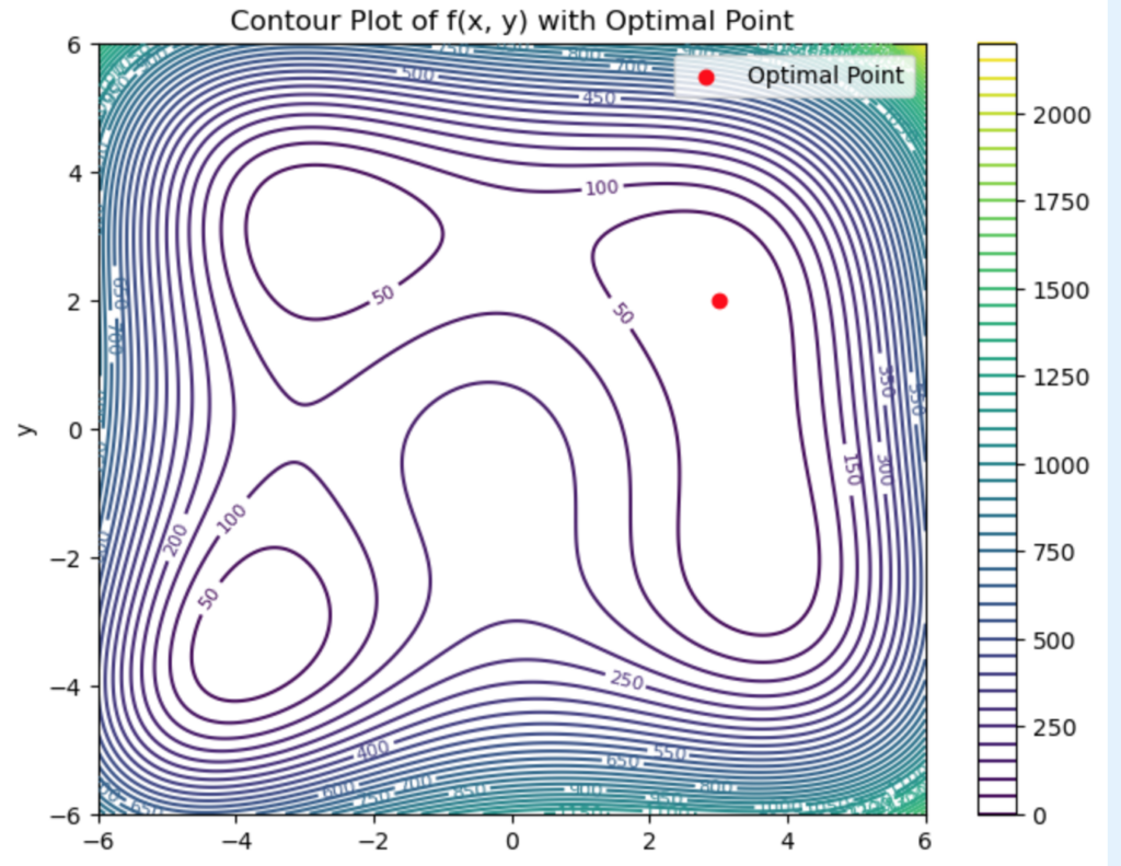
plt.figure(figsize=(8, 6))
contour = plt.contour(X, Y, Z, levels=50, cmap='viridis')
plt.clabel(contour, inline=True, fontsize=8)
plt.scatter(x_opt, y_opt, color='red', label='Optimal Point')
plt.title("Contour Plot of f(x, y) with Optimal Point")
plt.xlabel("x")
plt.ylabel("y")
plt.legend()
plt.colorbar(contour)
plt.show()

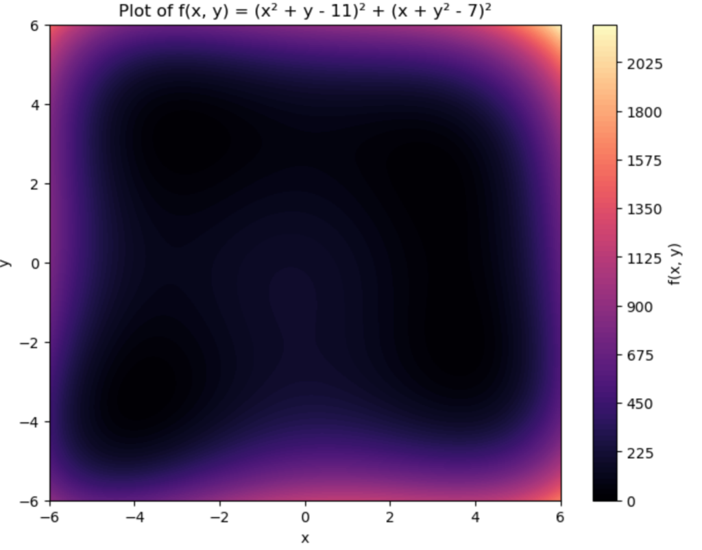
Now, lets try something that looks a little more exciting:

import numpy as np
import matplotlib.pyplot as plt

# Define the function
def f(x, y):
    return (x**2 + y - 11)**2 + (x + y**2 - 7)**2

# Generate a grid of x and y values
x = np.linspace(-6, 6, 500)
y = np.linspace(-6, 6, 500)
X, Y = np.meshgrid(x, y)
Z = f(X, Y)

# Plot the function
plt.figure(figsize=(8, 6))
plt.contourf(X, Y, Z, levels=100, cmap='magma')  # Gradient color
plt.colorbar(label='f(x, y)')
plt.title("Plot of f(x, y) = (x² + y - 11)² + (x + y² - 7)²")
plt.xlabel("x")
plt.ylabel("y")
plt.show()

That is cool looking.

Ok, lets take this even further:

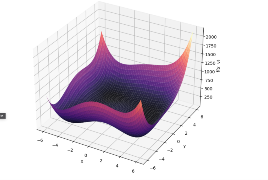
We can compare it to the Wolfram Function 3D plot:

from mpl_toolkits.mplot3d import Axes3D

# Create a 3D plot
fig = plt.figure(figsize=(10, 8))
ax = fig.add_subplot(111, projection='3d')

# Plot the surface
ax.plot_surface(X, Y, Z, cmap='magma', edgecolor='none', alpha=0.9)

# Labels and title
ax.set_title("3D Plot of f(x, y) = (x² + y - 11)² + (x + y² - 7)²")
ax.set_xlabel("x")
ax.set_ylabel("y")
ax.set_zlabel("f(x, y)")

plt.show()

Which gives you a 3D plot of the function:

3D Plot of f(x, y) = (x² + y – 11)² + (x + y² – 7)²

While this was a toy example for OpenMDAO, it is also a critical tool for advancing multidisciplinary optimization in engineering. Its robust capabilities, open-source nature, and focus on efficient computation of derivatives make it invaluable for researchers and practitioners seeking to tackle the complexities of modern system design.

i hope you find it useful.

Until Then,

#iwishyouwater <- The EDDIE – the most famous big wave contest ran this year. i saw it on the beach in 2004 and got washed across e rivermouth on a 60ft clean up set that washed out the river.

@tctjr

Music To Blog By: GodSpeedYouBlackEmperor “No Title As of 13 February 2024” – great band if you enjoy atmospheric compositional music.

SnakeByte[17] The Metropolis Algorithm

Frame Grab From the movie Metropolis 1927

Who told you to attack the machines, you fools? Without them you’ll all die!!

~ Grot, the Guardian of the Heart Machine

First, as always, Oh Dear Reader, i hope you are safe. There are many unsafe places in and around the world in this current time. Second, this blog is a SnakeByte[] based on something that i knew about but had no idea it was called this by this name.

Third, relative to this, i must confess, Oh, Dear Reader, i have a disease of the bibliomaniac kind. i have an obsession with books and reading. “They” say that belief comes first, followed by admission. There is a Japanese word that translates to having so many books you cannot possibly read them all. This word is tsundoku. From the website (if you click on the word):

“Tsundoku dates from the Meiji era, and derives from a combination of tsunde-oku (to let things pile up) and dokusho (to read books). It can also refer to the stacks themselves. Crucially, it doesn’t carry a pejorative connotation, being more akin to bookworm than an irredeemable slob.”

Thus, while perusing a math-related book site, i came across a monograph entitled “The Metropolis Algorithm: Theory and Examples” by C Douglas Howard [1].

i was intrigued, and because it was 5 bucks (Side note: i always try to buy used and loved books), i decided to throw it into the virtual shopping buggy.

Upon receiving said monograph, i sat down to read it, and i was amazed to find it was closely related to something I was very familiar with from decades ago. This finally brings us to the current SnakeByte[].

The Metropolis Algorithm is a method in computational statistics used to sample from complex probability distributions. It is a type of Markov Chain Monte Carlo (MCMC) algorithm (i had no idea), which relies on Markov Chains to generate a sequence of samples that can approximate a desired distribution, even when direct sampling is complex. Yes, let me say that again – i had no idea. Go ahead LazyWeb^TM laugh!

So let us start with how the Metropolis Algorithm and how it relates to Markov Chains. (Caveat Emptor: You will need to dig out those statistics books and a little linear algebra.)

Markov Chains Basics

A Markov Chain is a mathematical system that transitions from one state to another in a state space. It has the property that the next state depends only on the current state, not the sequence of states preceding it. This is called the Markov property. The algorithm was introduced by Metropolis et al. (1953) in a Statistical Physics context and was generalized by Hastings (1970). It was considered in the context of image analysis (Geman and Geman, 1984) and data augmentation (Tanner (I’m not related that i know of…) and Wong, 1987). However, its routine use in statistics (especially for Bayesian inference) did not take place until Gelfand and Smith (1990) popularised it. For modern discussions of MCMC, see e.g. Tierney (1994), Smith and Roberts (1993), Gilks et al. (1996), and Roberts and Rosenthal (1998b).

Ergo, the name Metropolis-Hastings algorithm. Once again, i had no idea.

Anyhow,

A Markov Chain can be described by a set of states $S$ and a transition matrix $P$ , where each element $P_{ij}$ represents the probability of transitioning from state $i$ to state $j$ .

Provide The Goal: Sampling from a Probability Distribution $\pi(x)$

In many applications (e.g., statistical mechanics, Bayesian inference, as mentioned), we are interested in sampling from a complex probability distribution $\pi(x)$ . This distribution might be difficult to sample from directly, but we can use a Markov Chain to create a sequence of samples that, after a certain period (called the burn-in period), will approximate $\pi(x)$ .

Ok Now: The Metropolis Algorithm

The Metropolis Algorithm is one of the simplest MCMC algorithms to generate samples from $\pi(x)$ . It works by constructing a Markov Chain whose stationary distribution is the desired probability distribution $\pi(x)$ . A stationary distribution is a probability distribution that remains the same over time in a Markov chain. Thus it can describe the long-term behavior of a chain, where the probabilities of being in each state do not change as time passes. (Whatever time is, i digress.)

The key steps of the algorithm are:

Initialization

Start with an initial guess $x_0$ , a point in the state space. This point can be chosen randomly or based on prior knowledge.

Proposal Step

From the current state $x_t$ , propose a new state $x^*$ using a proposal distribution $q(x^*|x_t)$ , which suggests a candidate for the next state. This proposal distribution can be symmetric (e.g., a normal distribution centered at $x_t$ ) or asymmetric.

Acceptance Probability

Calculate the acceptance probability $\alpha$ for moving from the current state $x_t$ to the proposed state $x^*$ :

$\alpha = \min \left(1, \frac{\pi(x^) q(x_t | x^)}{\pi(x_t) q(x^* | x_t)} \right)$

In the case where the proposal distribution is symmetric (i.e., $q(x^|x_t) = q(x_t|x^))$ , the formula simplifies to:

$\alpha = \min \left(1, \frac{\pi(x^*)}{\pi(x_t)} \right)$

Acceptance or Rejection

Generate a random number $u$ from a uniform distribution $U(0, 1)$
If $u \leq \alpha$ , accept the proposed state $x^*$ , i.e., $set x_{t+1} = x^*$ .
If $u > \alpha$ , reject the proposed state and remain at the current state, i.e., $set x_{t+1} = x_t$ .

Repeat

Repeat the proposal, acceptance, and rejection steps to generate a Markov Chain of samples.

Convergence and Stationary Distribution:

Over time, as more samples are generated, the Markov Chain converges to a stationary distribution. The stationary distribution is the target distribution $\pi(x)$ , meaning the samples generated by the algorithm will approximate $\pi(x)$ more closely as the number of iterations increases.

Applications:

The Metropolis Algorithm is widely used in various fields such as Bayesian statistics, physics (e.g., in the simulation of physical systems), machine learning, and finance. It is especially useful for high-dimensional problems where direct sampling is computationally expensive or impossible.

Key Features of the Metropolis Algorithm:

Simplicity: It’s easy to implement and doesn’t require knowledge of the normalization constant of $\pi(x)$ , which can be difficult to compute.
Flexibility: It works with a wide range of proposal distributions, allowing the algorithm to be adapted to different problem contexts.
Efficiency: While it can be computationally demanding, the algorithm can provide high-quality approximations to complex distributions with well-chosen proposals and sufficient iterations.

The Metropolis-Hastings Algorithm is a more general version that allows for non-symmetric proposal distributions, expanding the range of problems the algorithm can handle.

Now let us code it up:

i am going to assume the underlying distribution is Gaussian with a time-dependent mean $\mu_t$ , which changes slowly over time. We’ll use a simple time-series analytics setup to sample this distribution using the Metropolis Algorithm and plot the results. Note: When the target distribution is Gaussian (or close to Gaussian), the algorithm can converge more quickly to the true distribution because of the symmetric smooth nature of the normal distribution.

import numpy as np
import matplotlib.pyplot as plt

# Time-dependent mean function (example: sinusoidal pattern)
def mu_t(t):
    return 10 * np.sin(0.1 * t)

# Target distribution: Gaussian with time-varying mean mu_t and fixed variance
def target_distribution(x, t):
    mu = mu_t(t)
    sigma = 1.0  # Assume fixed variance for simplicity
    return np.exp(-0.5 * ((x - mu) / sigma) ** 2)

# Metropolis Algorithm for time-series sampling
def metropolis_sampling(num_samples, initial_x, proposal_std, time_steps):
    samples = np.zeros(num_samples)
    samples[0] = initial_x

    # Iterate over the time steps
    for t in range(1, num_samples):
        # Propose a new state based on the current state
        x_current = samples[t - 1]
        x_proposed = np.random.normal(x_current, proposal_std)

        # Acceptance probability (Metropolis-Hastings step)
        acceptance_ratio = target_distribution(x_proposed, time_steps[t]) / target_distribution(x_current, time_steps[t])
        acceptance_probability = min(1, acceptance_ratio)

        # Accept or reject the proposed sample
        if np.random.rand() < acceptance_probability:
            samples[t] = x_proposed
        else:
            samples[t] = x_current

    return samples

# Parameters
num_samples = 10000  # Total number of samples to generate
initial_x = 0.0      # Initial state
proposal_std = 0.5   # Standard deviation for proposal distribution
time_steps = np.linspace(0, 1000, num_samples)  # Time steps for temporal evolution

# Run the Metropolis Algorithm
samples = metropolis_sampling(num_samples, initial_x, proposal_std, time_steps)

# Plot the time series of samples and the underlying mean function
plt.figure(figsize=(12, 6))

# Plot the samples over time
plt.plot(time_steps, samples, label='Metropolis Samples', alpha=0.7)

# Plot the underlying time-varying mean (true function)
plt.plot(time_steps, mu_t(time_steps), label='True Mean ', color='red', linewidth=2)

plt.title("Metropolis Algorithm Sampling with Time-Varying Gaussian Distribution")
plt.xlabel("Time")
plt.ylabel("Sample Value")
plt.legend()
plt.grid(True)
plt.show()

Output of Python Script Figure 1.0

Ok, What’s going on here?

For the Target Distribution:

The function $mu_t(t)$ defines a time-varying mean for the distribution. In this example, it follows a sinusoidal pattern.
The function target_distribution(x, t) models a Gaussian distribution with mean $\mu_t$ and a fixed variance (set to 1.0).

Metropolis Algorithm:

The metropolis_sampling function implements the Metropolis algorithm. It iterates over time, generating samples from the time-varying distribution. The acceptance probability is calculated using the target distribution at each time step.

Proposal Distribution:

A normal distribution centered around the current state with standard deviation proposal_std is used to propose new states.

Temporal Evolution:

The time steps are generated using np.linspace to simulate temporal evolution, which can be used in time-series analytics.

Plot The Results:

The results are plotted, showing the samples generated by the Metropolis algorithm as well as the true underlying mean function $\mu_t$ (in red).

The plot shows the Metropolis samples over time, which should cluster around the time-varying mean $\mu_t$ of the distribution. As time progresses, the samples follow the red curve (the true mean) as time moves on like and arrow in this case.

Now you are probably asking “Hey is there a more pythonic library way to to this?”. Oh Dear Reader i am glad you asked! Yes There Is A Python Library! AFAIC PyMC started it all. Most probably know it as PyMc3 (formerly known as…). There is a great writeup here: History of PyMc.

We are golden age of probabilistic programming.

~ Chris Fonnesbeck (creator of PyMC)

Lets convert it using PyMC. Steps to Conversion:

Define the probabilistic model using PyMC’s modeling syntax.
Specify the Gaussian likelihood with the time-varying mean $\mu_t$ .
Use PyMC’s built-in Metropolis sampler.
Visualize the results similarly to how we did earlier.

import pymc as pm
import numpy as np
import matplotlib.pyplot as plt

# Time-dependent mean function (example: sinusoidal pattern)
def mu_t(t):
    return 10 * np.sin(0.1 * t)

# Set random seed for reproducibility
np.random.seed(42)

# Number of time points and samples
num_samples = 10000
time_steps = np.linspace(0, 1000, num_samples)

# PyMC model definition
with pm.Model() as model:
    # Prior for the time-varying parameter (mean of Gaussian)
    mu_t_values = mu_t(time_steps)

    # Observational model: Normally distributed samples with time-varying mean and fixed variance
    sigma = 1.0  # Fixed variance
    x = pm.Normal('x', mu=mu_t_values, sigma=sigma, shape=num_samples)

    # Use the Metropolis sampler explicitly
    step = pm.Metropolis()

    # Run MCMC sampling with the Metropolis step
    samples_all = pm.sample(num_samples, tune=1000, step=step, chains=5, return_inferencedata=False)

# Extract one chain's worth of samples for plotting
samples = samples_all['x'][0]  # Taking only the first chain

# Plot the time series of samples and the underlying mean function
plt.figure(figsize=(12, 6))

# Plot the samples over time
plt.plot(time_steps, samples, label='PyMC Metropolis Samples', alpha=0.7)

# Plot the underlying time-varying mean (true function)
plt.plot(time_steps, mu_t(time_steps), label='True Mean ', color='red', linewidth=2)

plt.title("PyMC Metropolis Sampling with Time-Varying Gaussian Distribution")
plt.xlabel("Time")
plt.ylabel("Sample Value")
plt.legend()
plt.grid(True)
plt.show()

When you execute this code you will see the following status bar:

It will be a while. Go grab your favorite beverage and take a walk…..

Output of Python Script Figure 1.1

Key Differences from the Previous Code:

PyMC Model Usage Definition:
In PyMC, the model is defined using the pm.Model() context. The x variable is defined as a Normal distribution with the time-varying mean $\mu_t$ . Instead of manually implementing the acceptance probability, PyMC handles this automatically with the specified sampler.

Metropolis Sampler:
PyMC allows us to specify the sampling method. Here, we explicitly use the Metropolis algorithm with pm.Metropolis().

Samples Parameter:
We specify shape=num_samples in the pm.Normal() distribution to indicate that we want a series of samples for each time step.

Plotting:
The resulting plot will show the sampled values using the PyMC Metropolis algorithm compared with the true underlying mean, similar to the earlier approach. Now, samples has the same shape as time_steps (in this case, both with 10,000 elements), allowing you to plot the sample values correctly against the time points; otherwise, the x and y axes would not align.

NOTE: We used this library at one of our previous health startups with great success.

Optimizations herewith include several. There is a default setting in PyMC which is called NUTS.
No need to manually set the number of leapfrog steps. NUTS automatically determines the optimal number of steps for each iteration, preventing inefficient or divergent sampling. NUTS automatically stops the trajectory when it detects that the particle is about to turn back on itself (i.e., when the trajectory “U-turns”). A U-turn means that continuing to move in the same direction would result in redundant exploration of the space and inefficient sampling. When NUTS detects this, it terminates the trajectory early, preventing unnecessary steps. Also the acceptance rates on convergence are higher.

There are several references to this set of algorithms. It truly a case of both mathematical and computational elegance.

Of course you have to know what the name means. They say words have meanings. Then again one cannot know everything.

Until Then,

#iwishyouwater <- Of all places Alabama getting the memo From Helene 2024

𝕋𝕖𝕕 ℂ. 𝕋𝕒𝕟𝕟𝕖𝕣 𝕁𝕣. (@tctjr) / X

Music To Blog By: View From The Magicians Window, The Psychic Circle

References:

[1] The Metropolis Algorithm: Theory and Examples by C Douglas Howard

[2] The Metropolis-Hastings Algorithm: A note by Danielle Navarro

[3] Github code for Sample Based Inference by bashhwu

Entire Metropolis Movie For Your Viewing Pleasure. (AFAIC The most amazing Sci-Fi movie besides BladeRunner)

November 10, 2020April 29, 2021 TCTJr Artificial_Intelligence|Complexity_Theory|Computational_Economics|Distributed_Computing

Computing The Human Condition – Project Noumena (Part 2)

In the evolution of a society, continued investment in complexity as a problem-solving strategy yields a declining marginal return.
Joseph A. Tainter

Someone asked me if from now on my blog will only be about Project_Noumena – on the contrary.

I will be interspersing subject matter within Parts 1 to (N) of Project_Noumena. To be transparent at this juncture i am not sure where it will end or if there is even a logical MVP 1.0. As with open-source systems and frameworks technically one never achieves V1.0 as the systems evolve. i tend to believe this will be the case with Project Noumena. i recently provided a book review on CaTB and have a blog on Recurrent Neural Networks with respect to Multiple Time Scale Prediction in the works so stuff is proceeding.

To that end, i would love comments and suggestions as to anything you would like my opinion on or for me to write about in the comments section. Also feel free to call me out on typos or anything else you see in error.

Further within Project Noumena there are snippets that could be shorter blogs as well. Look at Project Noumena as a fractal-based system.

Now on to the matter at hand.

In the previous blog Computing The Human_Condition – Project Noumena (Part 1) i discussed the initial overview of the model from the book World Dynamics. i will take a part of that model which is what i call, the main, Human_Do_Loop(); and the main attributes of the model: Birth and Death of Humans. One must ask if we didn’t have humans we would not have to be concerned with such matters as societal collapse? i don’t believe animals are concerned with such existential crisis concerns so my answer is a resounding – NO. We will be discussing such existential issues in this blog although i will address such items in future writings.

Over the years i have been asking myself is this a biological model by definition? Meaning do we have cellular components involved only? Is this biological modeling at the very essence? If we took the cell-based organisms out of the equation what do we still have as far as models on Earth?

While i told myself i wouldn’t get too extensional here and i do want to focus on the models and then codebases i continually check the initial conditions of these systems as they for most systems dictate the response for the rest of the future operations of said systems. Thus for biological systems, are there physical parameters that govern the initial exponential growth rate? Can we model with power laws and logistic curves for coarse-grained behavior? Is Bayesian reasoning biologically plausible at a behavioral level or at a neuronal level? Given that what are the atomic units that govern these models?

These are just a sampling of initial condition questions i ask myself as i evolve through this process.

So with that long-winded introduction and i trust i didn’t lose you oh reader lets hope into some specifics.

The picture from the book depicts basic birth and death loops in the population sector. In the case of these loops, they are generating positive feedback which causes growth. Thus an increase in population P causes an increase in birthrate BR. This, in turn, causes population P to further increase. The positive feedback loop would if left to its own devices would create an exponentially growing situation. As i said in the first blog and will continue to say, we seem to have started using exponential growth as a net positive fashion over the years in the technology industry. In the case of basic population dynamics with no constraints, exponential growth is not a net positive outcome.

Once again why start with simple models? The human mind is phenomenal at perceiving pressures, fears, greed, homeostasis, and other human aspects and characteristics and attempting at a structure that is given say the best fit to a situation and categorizing these as attributes thereof. However, the human mind is rather poor at predicting dynamical systems behaviors which are where the models come into play especially with social interactions and what i attempting to define from a self-organizing theory standpoint.

The next sets of loops that have the most effective behavior is a Pollution loop and a Crowding Loop. If we note that pollution POL increases one can assume up to a point that one hopes that nature absorbs and fixes the pollution otherwise it is a completely positive feedback loop and this, in turn, creates over pollution which we are already seeing the effects of around the worlds. One can then couple this with the amount of crowding humans can tolerate.

We see this behavior in urban sprawl areas when we have extreme heat or extreme cold or let’s say extreme pandemics. If the population rises crowding ratio increases the birth rate multiplier declines and birth rates reduce. The increasing death rate and reducing the birth rate are power system dynamic stabilizers coupled with pollution. This in turn obviously has an effect on food supplies. One can easily deduce that these seemingly simple coefficients if you will within the relative feedback loops create oscillations, exponential growth, or exponential decay. The systems while that seem large and rather stable are very sensitive to slight variations. If you are familiar with NetLogo it is a great agent-based modeling language. I picked a simple pollution model whereas we can select the number of people, birthrate, and tree planting rate.

As you can see without delving into the specifics after 77 years it doesn’t look to promising. i ‘ll either be using python or netlogo or a combination of both to extended these models as we add other references.

Ok enough for now.

Until Then,

#iwishyouwater

@tctjr

October 15, 2020October 16, 2020 TCTJr Books|Computational_Economics|Computing_History|Distributed_Computing|Human-Performance

Book Review: The Cathedral and The Bazaar (Musings On Linux and Open Source By An Accidental Revolutionary

“Joy, humor, and playfulness are indeed assets;”
~ Eric S. Raymond

As of late, i’ve been asked by an extreme set of divergent individuals what does “Open Source Software” mean?

That is a good question. While i understand the words and words do have meanings i am not sure its the words that matter here. Many people who ask me that question hear “open source” and hear or think “free’ which is not the case.

Also if you have been on linkedin at all you will see #Linux, #LinuxFoundation and #OpenSource tagged constantly in your feeds.

Which brings me to the current blog and book review.

(CatB)as it is affectionately known in the industry started out and still is a manifesto as well accessible via the world wide web. It was originally published in 1997 on the world wide wait and then in print form circa 1999. Then in 2001 was a revised edition with a foreword by Bob Young, the founding chairman and ceo of Redhat.

Being i prefer to use plain ole’ books we are reviewing the physical revised and extended paperback edition in this blog circa 2001. Of note for the picture, it has some wear and tear.

To start off as you will see from the cover there is a quote by Guy Kawasaki, Apple’s first Evangelist:

“The most important book about technology today, with implications that go far beyond programming.”

This is completely true. In the same train of thought, it even goes into the aspects of propriety and courtesy within conflict environments and how such environments are of a “merit not inherit” world, and how to properly respond when you are in vehement disagreement.

To relate it to the book review: What is a cathedral development versus a bazaar environment?

Cathedral is a tip of the fedora if you will to the authoritarian view of the world where everything is very structured and there are only a few at most who will approve moving the codebase forward.

Bazaar refers to the many. The many coding and contributing in a swarm like fashion.

In this book, closed source is described as a cathedral development model and open source as a bazaar development model. A cathedral is vertically and centrally controlled and planned. Process and governance rule the project – not coding. The cathedral is homeostatic. If you build or rebuild Basilica Sancti Petri within Roma you will not be picking it up by flatbed truck and moving it to Firenze.

The forward in the 2001 edition is written by Bob Young co-founder and original CEO of RedHat. He writes:

“ There have always been two things that would be required if open-source software was to materially change the world; one was for open-source software to become widely used and the other was the benefits this software development model supplied to its users had to be communicated and understood.”

Users here are an interesting target. Users could be developers and they could be end-users of warez. Nevertheless, i believe both conditions have been met accordingly.

i co-founded a machine learning and nlp service as a company in 2007 wherein i had the epiphany after my “second” read of Catb that the future is in fact open source. i put second in quotes as the first time i read it back in 1998 it wasn’t really a read in depth nor having fully internalized it while i was working at Apple in the CPU software department on OS9/OSX and while at the same time knowing full well that OSX was based on the Mach kernel. The Mach kernel is often mentioned as one of the earliest examples of a microkernel. However, not all versions of Mach are microkernels. Mach’s derivatives are the basis of the operating system kernel in GNU Hurd and of Apple’s XNU kernel used in macOS, iOS, iPadOS, tvOS, and watchOS.

That being said after years of working with mainly closed source systems in 2007 i re-read Catb. i literally had a deep epiphany that the future of all development would be open source distributed machine learning – everywhere.

Then i read it recently – deeply – a third time. This time nearly every line in the book resonates.

The third time with almost anything seems to be the charm. This third time through i realized not only is this a treatise for the open-source movement it is a call to arms if you will for the entire developer community to behave appropriately with propriety and courtesy in a highly matrixed collaborative environment known as the bazaar.

The most obvious question is: Why should you care? i’m glad you asked.

The reason you care is that you are part of the information economy. The top market cap companies are all information-theoretic developer-first companies. This means that these companies build things so others can build things. Software is truly eating the world. Think in terms of the recent pandemic. Work (code) is being created at an amazing rate due to the fact that the information work economy is distributed and essentially schedule free. She who has distributed wins and she who can code anytime wins. This also means that you are interested in building world-class software and the building of this software is now a decentralized peer reviewed transparent process.

The book is organized around Raymond’s various essays. It is important to note that just as software is an evolutionary process by definition so are the essays in this book. They can also be found online. The original collection of essays date back to 1992 on the internet: “A Brief History Of Hackerdom.’

The book is not a “how-to” cookbook but rather what i call a “why to” map of the terrain. While you can learn how to hack and code i believe it must be in your psyche. The book also uses the term “hacker” in a positive sense to mean one who creates software versus one who cracks software or steals information.

While the history and the methodology is amazing to me the cogent commentary on the types of the reasoning behind why hackers go into open source vary as widely as ice cream flavors.

Raymond goes into the theory of incentives with respect to the instinctive wiring of humans beings.

“The verdict of history seems to be free-market capitalism is the globally optimal way to cooperate for economic efficiency; perhaps in a similar way to cooperate for generating (and checking!) high-quality creative work.”

He categorizes command hierarchy, exchange economy, and gift culture to address these incentives.

Command hierarchy:

Goods are allocated in a scarce economy model by one central authority.

Exchange Economy:

The allocation of scarce goods is accomplished in a decentralized manner allowing scale through trade and voluntary cooperation.

Gift Culture:

This is very different than the other two methods or cultures. Abundance makes command and control relationships difficult to sustain. In gift cultures, social status is determined not by what you control but by what you give away.

It is clear that if we define the open source hackerdom it would be a gift culture. (It is beyond the current scope of this blog but it would be interesting to do a neuroscience project on the analysis of open source versus closed source hackers brain chemistry as they work throughout the day)

Given these categories, the essays then go onto define the written and many times unwritten (read secrets) that operate within the open-source world via a reputation game. If you are getting the idea it is tribal you are correct. Interestingly enough the open source world has in many cases very divergent views on all prickly things within the human condition such as religion and politics but one thing is a constant – ship high-quality code.

Without a doubt the most glaring cogent commentary comes in a paragraph from the essay “The Magic Cauldron.” entitled “Open Source And Strategic Business Risk.”

Ultimately the reasons open source seems destined to become a widespread practice have more to do with customer demand and market pressures than with supply-efficiencies for vendors.”

And further:

“Put yourself for the moment in the position of a CTO at a Fortune 500 corporation contemplating a build or upgrade of your firm’s IT infrastructure. Perhaps you need to choose a network operating system to be deployed enterprise-wide; perhaps your concerns involve 24/7 web service and e-commerce, perhaps your business depends on being able to field high-volume, high-reliability transaction databases. Suppose you go the conventional closed-source route. If you do, then you put your firm at the mercy of a supplier monopoly – because by definition there is only one place you can go to for support, bug fixes, and enhancements. If the supplier doesn’t perform, you will have no effective recourse because you are effectively locked by your initial investment.”

FURTHER:

“The truth is this: when your key business processes are executed by opaque blocks of bits that you cant even see inside (let alone modify) you have lost control of your business.”

“Contrast this with the open-source choice. If you go this route, you have the source code, and no one can take that away from you. Instead of a supplier monopoly with a choke-hold on your business, you now have multiple service companies bidding for your business – and you not only get to play them against each other, but you also have the option of building your own captive support organization if that looks less expensive than contracting out. The market works for you.”

“The logic is compelling; depending on closed-source code is an unacceptable strategic risk So much so that I believe it will not be very long until closed-source single-vendor acquisitions when there is an open source alternative available will be viewed as a fiduciary irresponsibility, and rightly grounds for a share-holder lawsuit.”

THIS WAS WRITTEN IN 1997. LOOK AROUND THE WORLD WIDE WAIT NOW… WHAT DO YOU SEE?

Open Source – full stop.

i will add that there was no technical explanation here only business incentive and responsibility to the company you are building, rebuilt, or are scaling. Further, this allows true software malleability and reach which is the very reason for software.

i will also go on a limb here and say if you are a software corporation one that creates software you can play the monopoly and open-source models against each other within your corporation. Agility and speed to ship code is the only thing that matters these days. Where is your github? Or why is this not shipping TODAY?

This brings me to yet another amazing prescient prediction in the book that Raymond says that applications are ultimately where we will land for monetary scale. Well yes, there is an app for that….

While i have never met Eric S. Raymond he is a legend in the field. We have much to thank him for in the areas of software. If you have not read CatB and work in the information sector do yourself a favor: buy it today.

As a matter of fact here is the link: The Cathedral & the Bazaar: Musings on Linux and Open Source by an Accidental Revolutionary

Muzak To Blog To: “Morning Phase” by Beck

Resources:

http://www.opensource.org

https://www.apache.org/foundation/

Computing The Human Condition – Project Noumena (Part 1)

“I am putting myself to the fullest possible use, which is all I think any conscious entity can ever hope to do.” ~ HAL 9000

“If you want to make the world a better place take a look at yourself and then make a change.” ~ MJ.

First and foremost with this blog i trust everyone is safe. The world is in an interesting place, space, and time both physically and dare i say collectively – mentally.

Introduction

This past week we celebrated Earth Day. i believe i heard it was the 50th year of Earth Day. While I applaud the efforts and longevity for a day we should have Earth Day every day. Further just “thoughting” about or tweeting about Earth Day – while it may wake up your posterior lobe of the pituitary gland and secret some oxytocin – creating the warm fuzzies for you it really doesn’t create an action for furthering Earth Day. (much like typing /giphy YAY! In Slack).

As such, i decided to embark on a multipart blog that i have been “thinking” about what i call an Ecological Computing System. Then the more i thought about it why stop at Ecology? We are able to model and connect essentially anything, we now have models for the brain that while are coarse-grained can account for gross behaviors, we have tons of data on buying habits and advertisement data and everything is highly mobile and distributed. Machine learning which can optimize, classify and predict with extremely high dimensionality is no longer an academic exercise.

Thus, i suppose taking it one step further from ecology and what would differentiate it from other efforts is that <IT> would actually attempt to provide a compute framework that would compute The Human Condition. I am going to call this effort Project Noumena. Kant the eminent thinker of 18th century Germany defined Noumena as a thing as it is in itself, as distinct from a thing as it is knowable by the senses through phenomenal attributes and proposed that the experience was a product of the mind.

My impetus for this are manifold:

i love the air, water, trees, and animals,

i am an active water person,

i want my children’s children’s children to know the wonder of staring at the azure skies, azure oceans and purple mountains,

Maybe technology will assist us in saving us from The Human Condition.

Timing

i have waited probably 15+ years to write about this ideation of such a system mainly due to the technological considerations were nowhere near where they needed to be and to be extremely transparent no one seemed to really think it was an issue until recently. The pandemic seems to have been a global wakeup call that in fact, Humanity is fragile. There are shortages of resources in the most advanced societies. Further due to the recent awareness that the pollution levels appear (reported) to be subsiding as a function in the reduction of humans’ daily involvement within the environment. To that point over the past two years, there appears to be an uptake of awareness in how plastics are destroying our oceans. This has a coupling effect that with the pandemic and other environmental concerns there could potentially be a food shortage due to these highly nonlinear effects. This uptake in awareness has mainly been due to the usage of technology of mobile computing and social media which in and of itself probably couldn’t have existed without plastics and massive natural resource consumption. So i trust the irony is not lost there.

From a technical perspective, Open source and Open Source Systems have become the way that software is developed. For those that have not read The Cathedral and The Bazaar and In The Beginning Was The Command Line i urge you to do so it will change your perspective.

We are no longer hampered by the concept of scale in computing. We can also create a system that behaves at scale with only but a few human resources. You can do a lot with few humans now which has been the promise of computing.

Distributed computing methods are now coming to fruition. We no longer think in terms of a monolithic operating system or in place machine learning. Edge computing and fiber networks are accelerating this at an astonishing rate. Transactions now dictate trust. While we will revisit this during the design chapters of the blog I’ll go out on a limb here and say these three features are cogent to distributed system processing (and possibly the future of computing at scale).

Incentive models
Consensus models
Protocol models

We will definitely be going into the deeper psychological, mathematical, and technical aspects of these items.

Some additional points of interest and on timing. Microsoft recently released press about a Planetary Computer and announced the position of Chief Ecology Officer. While i do not consider Project Nuomena to be of the same system type there could be similarities on the ecological aspects which just like in open source creates a more resilient base to work.

The top market cap companies are all information theoretic-based corporations. Humans that know the science, technology, mathematics and liberal arts are key to their success. All of these companies are woven and interwoven into the very fabric of our physical and psychological lives.

Thus it is with the confluence of these items i believe the time is now to embark on this design journey. We must address the Environment, Societal factors and the model of governance.

A mentor once told me one time in a land far away: “Timing is everything as long as you can execute.” Ergo Timing and Execution Is Everything.

Goals

It is my goal that i can create a design and hopefully, an implementation that is utilizing computational means to truly assist in building models and sampling the world where we can adhere to goals in making small but meaningful changes that can be used within what i am calling the 3R’s: recycle, redact, reuse. Further, i hope with the proper incentive models in place that are dynamic it has a mentality positive feedback effect. Just as in complexity theory a small change – a butterfly wings – can create hurricanes – in this case positive effect.

Here is my overall plan. i’m not big on the process or gant charts. I’ll be putting all of this in a README.md as well. I may ensconce the feature sets etc into a trello or some other tracking mechanism to keep me focused – WebSphere feel free to make recommendations in the comments section:

Action Items:

Create Comparative Models

Create Coarse-Grained Attributes

Identify underlying technical attributes

Attempt to coalesce into an architecture

Start writing code for the above.

Preamble

Humanity has come to expect growth as a material extension of human behavior. We equate growth with progress. In fact, we use the term exponential growth as it is indefinitely positive. In most cases for a fixed time interval, this means a doubling of the relevant system variable or variables. We speak of growth as a function of gross national production. In most cases, exponential growth is treacherous where there are no known or perceived limits. It appears that humanity has only recently become aware that we do not have infinite resources. Psychologically there is a clash between the exponential growth and the psychological or physical limit. The only significance is the relevant (usually local) limit. How does it affect me, us, and them? This can be seen throughput most game theory practices – dominant choice. The pattern of growth is not the surprise it is the collision of the awareness of the limit to the ever-increasing growth function is the surprise.

One must stop and ask:

Q: Are progress (and capacity) and the ever-increasing function a positive and how does it relate to 2nd law of thermodynamics aka Entropy? Must it always expand?

We are starting to see that our world can exert dormant forces that within our life can greatly affect our well being. When we approach the actual or perceived limit the forces which are usually negative begin to gain strength.

So given these aspects of why i’ll turn now to start the discussion. If we do not understand history we cannot predict the future by inventing it or in most cases re-inventing it as it where.

I want to start off the history by referencing several books that i have been reading and re-reading on subjects of modeling the world, complexity, and models for collapse throughout this multipart blog. We will be addressing issues concerning complex dynamics as are manifested with respect to attributes model types, economics, equality, and mental concerns.

These core references are located at the end of the blog under references. They are all hot-linked. Please go scroll and check them out. i’ll still be here. i’ll wait.

Checked them out? i know a long list.

As you can see the core is rather extensive due to the nature of the subject matter. The top three books are the main ones that have been the prime movers and guides of my thinking. These three books i will refer to as The Core Trilogy:

World Dynamics

The Collapse of Complex Societies

Six Sources of Collapse

As i mentioned i have been deeply thinking about all aspects of this system for quite some time. I will be mentioning several other texts and references along the continuum of creation of this design.

We will start by referencing the first book: World Dynamics by J.W. Forrestor. World Dynamics came out of several meetings of the Rome Club a 75 person invite-only club founded by the President of Fiat. The club set forth the following attributes for a dynamic model that would attempt to predict the future of the world:

Population Growth

Capital Investment

Geographical Space

Natural Resources

Pollution

Food Production

The output of this design was codified in a computer program called World3. It has been running since the 1970s what was then termed a golden age of society in many cases. All of these variables have been growing at an exponential rate. Here we see the model with the various attributes in action. There have been several criticisms of the models and also analysis which i will go into in further blogs. However, in some cases, the variants have been eerily accurate. The following plot is an output of the World3 model:

Issues Raised By World3 and World Dynamics

The issues raised by World3 and within the book World Dynamics are the following:

There is a strong undercurrent that technology might not be the savior of humankind

Industrialism (including medicine and public health) may be a more disturbing force than the population.

We may face extreme psychological stress and pressures from a four-pronged dilemma via suppression of the modern industrial world.

We may be living in a “golden age” despite a widely acknowledged feeling of malaise.

Exhtortions and programs directed at population control may be self-defeating. Population control, if it works, would yield excesses thereby allowing further procreation.

Pollution and Population seem to oscillate whereas the high standard of living increases the production of food and material goods which outrun the population. Agriculture as it hits a space limit and as natural resources reach a pollution limit then the quality of life falls in equalizing population.

There may be no realistic hope of underdeveloped countries reaching the same standard and quality of life as developed countries. However, with the decline in developed countries, the underdeveloped countries may be equalized by that decline.

A society with a high level of industrialization may be unsustainable.

From a long term 100 years hence it may be unwise for underdeveloped countries to seek the same levels of industrialization. The present underdeveloped nations may be in better conditions for surviving the forthcoming pressures. These underdeveloped countries would suffer far less in a world collapse.

Fuzzy Human – Fuzzy Model

The human mind is amazing at identifying structures of complex situations. However, our experiences train us poorly for estimating the dynamic consequences of said complexities. Our mind is also not very accurate at estimating ad hoc parts of the complexities and the variational outcomes.

One of the problems with models is well it is just a model The subject-observer reference could shift and the context shifts thereof. This dynamic aspect needs to be built into the models.

Also while we would like to think that our mental model is accurate it is really quite fuzzy and even irrational in most cases. Also attempting to generalize everything into a singular model parameter is exceedingly difficult. It is very difficult to transfer one industry model onto another.

In general parameterization of most of these systems is based on some perceptual model we have rationally or irrationally invented.

When these models were created there was the consideration of modeling social mechanics of good-evil, greed – altruism, fears, goals, habits, prejudice, homeostasis, and other so-called human characteristics. We are now at a level of science where we can actually model the synaptic impulse and other aspects that come with these perceptions and emotions.

There is a common cross-cutting construct in most complex models within this text that consists of and mainly concerned with the concept of feedback and how the non-linear relationships of these modeled systems feedback into one another. System-wide thinking permeates the text itself. On a related note from the 1940’s of which Dr Norbert Weiner and others such as Claude Shannon worked on ballistic tracking systems and coupled feedback both in a cybernetic and information-theoretic fashion of which he attributed the concept of feedback as one of the most fundamental operations in information theory. This led to the extremely famous Weiner Estimation Filters. Also, side note: Dr Weiner was a self-styled pacifist proving you can hold two very opposing views in the same instance whilst being successful at executing both ideals.

Given that basic function of feedback, lets look at the principle structures. Essentially the model states there will be levels and rates. Rates are flows that cause levels to change. Levels can accumulate the net level. Either addition or subtraction to that level. The various system levels can in aggregate describe the system state at any given time $(t)$ . Levels existing in all subsystems of existence. These subsystems as you will see include but are not limited to financial, psychological, biological, and economic. The reason that i say not limited to because i also believe there are some yet to be identified subsystems at the quantum level. The differential or rate of flow is controlled by one or more systems. All systems that have some Spatio-temporal manifestation can be represented by using the two variables levels and rates. Thus with respect to the spatial or temporal variables, we can have a dynamic model.

The below picture is the model that grew out of interest from the initial meetings of the Club of Rome. The inaugural meeting which was the impetus for the model was held in Bern, Switzerland on June 29, 1970. Each of the levels presents a variable in the previously mentioned major structures. System levels appear as right triangles. Each level is increased or decreased by the respective flow. As previously mentioned on feedback any closed path through the diagram is a feedback loop. Some of the closed loops given certain information-theoretic attributes be positive feedback loops that generate growth and others that seek equilibrium will be negative feedback loops. If you notice something about the diagram it essentially is a birth and death loop. The population loop if you will. For the benefit of modeling, there are really only two major variables that affect the population. Birth Rate (BR) and Death Rate (DR). They represent the total aggregate rate at which the population is being increased or decreased. The system has coefficients that can initialize them to normal rates. For example, in 1970 BRN is taken as 0.0885 (88.5 per thousand) which is then multiplied by population to determine BR. DRN by the same measure is the outflow or reduction. In 1970 it was 9.5% or 0.095. The difference is the net and called normal rates. The normale rates correspond to a physical normal world. When there are normal levels of food, material standard of living, crowding, and pollution. The influencers are then multipliers that increase or decrease the normal rates.

As a caveat, there have been some detractors of this model. To be sure it is very coarse-grained however while i haven’t seen the latest runs or outputs it is my understanding as i said the current outputs are close. The criticisms come in the shape of “Well its just modeling everything as a $y=x*e^{{rt}}$ . I will be using this concept and map if you will as the basis for Noumena. The concepts and values as i evolve the system will vary greatly from the World3 model but i believe starting with a minimum viable product is essential here as i said humans are not very good at predicting all of the various outcomes in high dimensional space. We can asses situations very quickly but probably outcomes no so much. Next up we will be delving into the loops deeper and getting loopier.