Mathematics | Theodore C. Tanner Jr.

Pre-Computing War

Sora’s idea of a Neon Drone War With Audio Track

Sometimes it is the people no one can imagine anything of who do the things no one can imagine.

~ Alan Turing

First, i trust everyone is safe. Second, i had a creative spurt of late and wrote the following blog in one sitting after waking up thinking about the subject.

NOTE: This post is in no way indicative of any stance or provides any classified information whatsoever. It is only a thought piece concerning current technology-driven areas of concern.

Preamble

There is a paradigm shift happening that will affect future generations and possibly the very essence of what it means to be human, and this comes from how technology is transforming war. We stand at a precipice, gazing into a future where the tools of war no longer resemble the clashing steel and human courage of centuries past. How important is conflict to humanity? What is the essence and desire for this conflict? The current uptick in drone usage of the past years has created an inflection point for what I am terming “abstraction levels for engagement.”

We continue to underestimate how important drones are going to be in warfare—a miscalculation that echoes through history’s long ledger of missed signals. I’m going to go out on a long limb here and say the future of most warfare will be enabled by, driven by, and spearheaded by drones. In fact, other than some other types of autonomous vehicles, there might not be anything else on the battlefield.

Here is a definition (of course, AI bot generated because really who reads Webster’s Dictionary nowadays? For the record, i have read Webster’s 3 times front to back):

“A military drone, also known as an unmanned aerial vehicle (UAV) or unmanned aircraft system (UAS), is an aircraft flown without a human pilot on board, controlled remotely or autonomously, and used for military missions like surveillance, reconnaissance, and potentially combat operations. “

This isn’t hyperbole; it’s the logical endpoint of a trajectory we’ve been on since the first unmanned systems took flight. And at the end of that trajectory lies something even more radical: autonomous bullets—not merely guided, but self-directed, a fusion of machine intelligence and lethal intent that could redefine conflict itself.

Note: I edited this part as the kind folk on The LazyWeb(tm) were laser-focused on the how of “smart bullets.: Great feedback and thank you. git push -u -f origin main.

Guided autonomous bullets, often referred to as “smart bullets,” represent an advanced leap in projectile technology, blending precision guidance systems with small-caliber ammunition. These bullets are designed to adjust their flight path mid-air to hit a target with exceptional accuracy, even if the target is moving or environmental factors like wind interfere. The concept builds on precision guided munitions used in larger systems like missiles, but shrinks the technology to fit within the constraints of a bullet fired from a firearm.

Autonomous bullets, often referred to as “smart bullets,” are advanced projectiles designed to adjust their trajectory mid-flight to hit a target with high precision, even under challenging conditions like wind or a moving target. While the concept might sound like science fiction, significant research has been conducted, particularly by organizations like DARPA (Defense Advanced Research Projects Agency) and Sandia National Laboratories, to make this technology a reality.

The core idea behind autonomous bullets is to integrate guidance systems into small-caliber projectiles, allowing them to self-correct their path after being fired. One of the earliest designs, as described in “historical research”, involved a bullet with three fiber-optic sensors (or “eyes”) positioned around its circumference to provide three-dimensional awareness. A laser is used to designate the target, and as the bullet travels, these sensors detect the laser’s light. The bullet adjusts its flight path in real time to ensure an equal amount of laser light enters each sensor, effectively steering itself toward the laser-illuminated target. This method prevents the bullet from making drastic turns like a missile. Still, it enables small, precise adjustments to hit exactly where the laser is pointed, even if the target is beyond visual range or the laser source is separate from the shooter. It hath been said that if you can think it DARPA has probably built it, maybe.

Given the advancements in drones, unmanned autonomous vehicles, land and air vehicles, and supposedly smart bullets (only the dark web knows how they work), imagine a battlefield stripped of human presence, not out of cowardice but necessity. The skies a deafening hum with swarms of drones (if a drone makes a sound and no one is there to hear it, does it make a sound?), each a “node” orchestrated via particle swarm AI models in a vast, decentralized network of artificial minds.

No generals barking orders, no soldiers trudging through mud, just silicon and steel executing a dance of destruction with precision beyond human capacity. The end state of drones isn’t just remote control or pre-programmed strikes; it’s autonomy so complete that the machines themselves decide who lives and who dies – no human in the loop. Self-directed projectiles, bullets with brains roaming the theater of war, seeking targets based on algorithms fed by real-time data streams. The vision feels like science fiction, yet the pieces already fall into place.

Generals gathered in their masses
just like witches at black masses
evil minds that plot destruction
sorcerers of death’s construction
in the fields the bodies burning
as the war machine keeps turning
death and hatred to mankind
poisoning their brainwashed minds, oh lord yeah!

~ War Pigs, Black Sabbath 1970

This shift isn’t merely tactical; it’s existential. Warfare has always been a contest of wills, a brutal arithmetic of resources and resolve. But what happens when we can compute the outcome before the first shot is fired? Drones, paired with advanced AI, offer the tantalizing possibility of simulating conflicts down to the last variable terrain, weather, enemy morale, and supply lines, all processed in milliseconds by systems that learn as they go. The autonomous bullet isn’t just a weapon; it’s a data point in a larger Markovian equation, one that could predict victory or defeat with chilling accuracy.

We’re not far from a world where wars are fought first in the cloud, their outcomes modeled and refined, before a single drone lifts off.If the future of warfare is of drone swarms of autonomous systems culminating in self-directed bullets, then pre-computing its outcomes becomes not just feasible but imperative. The battlefield of tomorrow isn’t a chaotic melee; it’s a high-stakes game, a multidimensional orchestrated chessboard where game theory, geopolitics, and macroeconomics converge to predict the endgame before the first move. To compute warfare in this way requires us to distill its essence into variables, probabilities, and incentives a task as daunting as it is inevitable. Yet again, there exists a terminology for this orchestrated chess game. Autonomous asymmetric mosaic warfighting, a concept explored by DARPA, envisions turning complexity into an asymmetric advantage by using networked, smaller, and less complex systems to overwhelm an adversary with a multitude of capabilitiesnvisions turning complexity into an asymmetric advantage by using networked, smaller, and less complex systems to overwhelm an adversary with a multitude of capabilities.

“A Nash equilibrium is a set of strategies that players act out, with the property that no player benefits from changing their strategy. ~ Dr John Nash.”

Computational Game Theory: The Logic of Lethality

At its core, warfare is a strategic interaction, a contest where players, nations, factions, or even rogue actors vie for dominance under the constraints of resources and information. Game theory offers the scaffolding to model this. Imagine a scenario where drones dominate: each side deploys autonomous swarms, programmed with decision trees that weigh attack, retreat, or feint based on real-time data. The payoff matrix isn’t just about territory or casualties, it’s about disruption, deterrence, and psychological impact. A swarm’s choice to strike a supply line rather than a command center could shift an enemy’s strategy, forcing a cascade of recalculations.

Now, introduce autonomous bullets, self-directed agents within the swarm. Each bullet becomes a player in a sub-game, optimizing its path to maximize damage while minimizing exposure. The challenge lies in anticipating the opponent’s moves: if both sides rely on AI-driven systems, the game becomes a duel of algorithms, each trying to out-predict the other. Zero-sum models give way to dynamic equilibria, where outcomes hinge on how well each side’s AI can bluff, adapt, or exploit flaws in the other’s logic. Pre-computing this requires vast datasets, historical conflicts, behavioral patterns, and even cultural tendencies fed into simulations that run millions of iterations, spitting out probabilities of victory, stalemate, or collapse.

Geopolitics: The Board Beyond the Battlefield

Warfare doesn’t exist in a vacuum; the shifting tectonic plates of geopolitics shape it. To pre-compute outcomes, we must map the global chessboard—alliances, rivalries, and spheres of influence. Drones level the playing field, but their deployment reflects deeper asymmetries. A superpower with advanced AI and manufacturing might flood the skies with swarms, while a smaller state leans on guerrilla tactics, using cheap, hacked drones to harass and destabilize. The game-theoretic model expands: players aren’t just combatants but also suppliers, proxies, and neutral powers with their own agendas.

Take energy as a (the main) variable: drones require batteries, rare earths, and infrastructure. A nation controlling lithium mines or chip fabs holds leverage, tipping the simulation’s odds. Sanctions, trade routes, and cyber vulnerabilities—like a rival hacking your drone fleet’s firmware—become inputs in the equation. Geopolitical stability itself becomes a factor: if a war’s outcome hinges on a fragile ally, the model must account for the likelihood of defection or collapse. Pre-computing warfare here means forecasting not just the battle, but the ripple effects—will a decisive drone strike trigger a refugee crisis, a shift in NATO’s posture, or a scramble for Arctic resources? The algorithm must think in networks, not lines.

I visualize a time when we will be to robots what dogs are to humans, and I’m rooting for the machines.

~ Claude Shannon

Macroeconomics: The Sinews of Silicon War

No war is won without money, and drones don’t change that; they just rewrite the budget. Pre-computing conflict demands a macroeconomic lens: how much does it cost to field a swarm versus defend against one? The economics of autonomous warfare favor scale mass-produced drones and bullets could outpace legacy systems like jets or tanks in cost-efficiency. A simulation might pit a 10 billion dollar defense budget against a 1 billion dollar insurgent force, factoring in production rates, maintenance, and the price of countermeasures like EMPs or jamming tech.

But it’s not just about direct costs. Markets react to war’s shadow oil spikes, currencies wobble, tech stocks soar or crash based on who controls the drone supply chain (it is all about that theta/beta folks). A protracted conflict could drain a nation’s reserves, while a swift, computed victory might bolster its credit rating. The model must integrate these feedback loops: if a drone war craters a rival’s economy, their ability to replenish dwindles, tilting the odds. And what of the peacetime economy? States that mastering autonomous tech could dominate postwar reconstruction, turning military R&D into a geopolitical multiplier. Pre-computing this requires economic forecasts layered atop the game-theoretic core—GDP growth, inflation, and consumer confidence as resilience proxies.

The Supreme Lord said: I am mighty Time, the source of destruction that comes forth to annihilate the worlds. Even without your participation, the warriors arrayed in the opposing army shall cease to exist.~ Bhagavad Gita 11:32

The Synthesis: Simulating the Unthinkable

To tie it all together, picture a supercomputer or a distributed AI network running a grand simulation. It ingests game-theoretic strategies (strike patterns, bluffing probabilities), geopolitical alignments (alliances, resource choke points), and macroeconomic trends (war budgets, trade disruptions). Drones and their autonomous bullets are the pawns, but the players are human decision-makers, constrained by politics and profit. The system runs countless scenarios: a drone swarm cripples a port, triggering a naval response, spiking oil prices, and collapsing a coalition. Another sees a small state’s cheap drones hold off a giant, forcing a negotiated peace.

The output isn’t a single prediction, but a spectrum 75% chance of victory if X holds, 40% if Y defects, 10% if the economy tanks. Commanders could tweak inputs more drones, better AI, a preemptive cyberstrike and watch the probabilities shift. It’s not infallible; black swans like a rogue AI bug or a sudden uprising defy the math. But it’s close enough to turn war into a science, reducing the fog Clausewitz warned of to a manageable haze [1].

The thing that hath been, it is that which shall be; and that which is done is that which shall be done: and there is no new thing under the sun.

~ Ecclesiastes 1:9, KJV

Yet, this raises a haunting question: If we can compute warfare’s endgame, do we lose something essential in the process?

The chaos of flawed, emotional, unpredictable human decision-making has long been the wildcard that defies calculation. Napoleon’s audacity, the Blitz’s resilience, and the guerrilla fighters’ improvisation are not easily reduced to code. Drones and their self-directed progeny promise efficiency, but they also threaten to strip war of its human texture, turning it into a sterile exercise in optimization. And what of accountability? When a bullet chooses its target, who bears the moral weight—the coder, the commander, or the machine itself?

The implications stretch beyond the battlefield. If drones dominate warfare, the barriers to entry collapse. No longer will nations need vast armies or industrial might; a few clever engineers and a swarm of cheap, autonomous systems could level the playing field. We’ve seen glimpses of this in Ukraine, where off-the-shelf drones have humbled tanks and disrupted supply lines. Scale that up, and the future isn’t just drones it’s a proliferation of power, a democratization of destruction. Autonomous bullets could become the ultimate equalizer or the ultimate chaos agent, depending on who wields them.

Fighting for peace is like screwing for virginity.

~ George Carlin

A Moment of Clarity

i wonder: are we ready to surrender the reins? The dream of computing warfare’s outcome is seductive and humans are carnal creatures we lust for other humans and things, thus it promises to minimize loss, to replace guesswork with certainty, but it also risks turning us into spectators of our own fate, watching as machines play out scenarios we’ve set in motion (that which we lust after).

The end state of drones may indeed be a battlefield of self-directed systems, but the end state of humanity in that equation remains unclear. Perhaps the true revolution isn’t in the technology but in how we grapple with a world where war becomes a problem to be solved rather than a story to be lived.

We underestimate drones at our peril. They’re not just tools; they’re harbingers of a paradigm shift. The future is coming, and it’s buzzing overhead—relentless, autonomous, and utterly indifferent to our nostalgia for the wars of old.

Pre-computing warfare might make us too confident. Leaders who trust the model might rush to conflict, assuming the odds are locked. But humans aren’t algorithms; we rebel, err, and surprise. And what of ethics? A simulation that optimizes for victory might greenlight drone strikes on civilians to break morale, justified by a percentage point. The autonomous bullet doesn’t care; it’s our job to decide if the computation is worth the soul it costs.

In this drone-driven future, pre-computing warfare isn’t just possible—it’s already beginning. Ukraine’s drone labs, China’s swarm tests, the Pentagon’s AI budgets—they’re all steps toward a world where conflict is a solvable problem. It has been said that fighting and sex are the two book ends but one in the same. But as we build the machine to predict the fight, we must ask: are we mastering war, or merely handing it a new master for something else entirely?

Music To Blog By: Project-X “Closing Down The Systems. Actually, I wouldn’t listen to this if i were you, unless you want to have nightmares. Fearless (MZ412 Remix) does sound like computational warfare.

Until then,

#iwishyouwater <- recent raw Pipe footage of folks that got the memo.

Ted ℂ. Tanner Jr. (@tctjr) / X

References:

[1] “On War” by Carl von Clausewitz. He called it “The Fog of War”: Clausewitz stressed the importance of understanding the unpredictable nature of war, noting that the “fog of war” (i.e., incomplete, dubious, and often erroneous information and great fear, doubt, and excitement) can lead to rapid decisions by alert commanders.

[2] Thanks to Jay Sales for being the catalyst for this blog. If you do not know who he is look him up here. Jay Sales. One of the best engineering executives and dear friend.

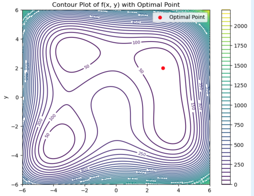
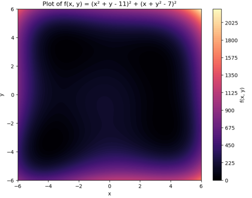
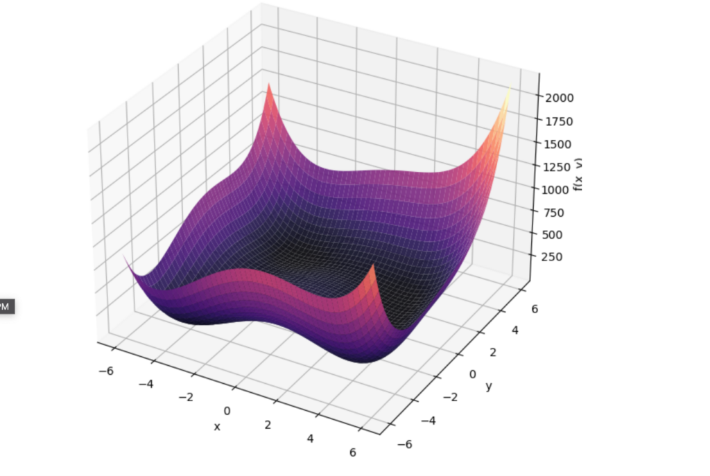
NVIDIA GTC 2025: The Time Has Come The Valley Said

OpenAI’s idea of The Valley – Its Been A Minute

Embrace the unknown and embrace change. That’s where true breakthroughs happen.

~Jensen Huang

First i trust everyone is safe. Second i usually do not write about discrete events or “work” related items but this is an exception. March 17-21, 2025 i and some others attended NVIDIA GTC2025. It warranted a long writeup. Be Forewarned: tl;dr. Read on Dear Reader. Hope you enjoy this one as it is a sea change in computing and a tectonic ocean shift in technology.

NVIDIA GTC 2025: AI’s Raw Hot Buttered Future

March 17-21, 2025, San Jose became geek central for NVIDIA’s GTC—aka the “Super Bowl of AI.” Hybrid setup, in-person or virtual, didn’t matter; thousands of devs, researchers, and suits swarmed to see what’s cooking in AI, GPUs, and robotics. Jensen Huang dropped bombs in his keynote, 1,000+ sessions drilled into the guts of it, and big players flexed their wares. Here’s the raw dog buttered scoop—and why you should care if you sling code or ship product.

The time has come,’ the Walrus said,

      To talk of many things:

Of shoes — and ships — and sealing-wax —

      Of cabbages — and kings —

And why the sea is boiling hot —

      And whether pigs have wings.’

~ The Walrus and The Carpenter

All The Libraries

Jensen’s Keynote: AI’s Next Gear, No Hype

March 18, 2025 SAP Center and the MCenery Civic Center, over 28,000 geeks packed in both halls and out in the streets . Jensen Huang, NVIDIA’s leather-jacketed maestro, hit the stage and didn’t waste breath. 2.5 hours no notes and started with the top of the stack with all the libraries NVIDIA has “CUDA-ized” and went all the way down to the photonic ethernet cables. No corporate fluff, just tech meat for the developer carnivore. His pitch: AI’s not just chatbots anymore; it’s “agentic,” thinking and moving in the real world forward at the speed of thought. Backed up with specifications, cycles, cost and even calling out library function calls.

Here’s what he unleashed:

Blackwell Ultra (B300): Mid-cycle beast, 288GB memory, out H2 2025. Training LLMs that’d choke lesser rigs—AMD’s sniffing, but NVIDIA’s still king.
Rubin + Vera Rubin: GPU + CPU superchip combo, late 2026. Named for the galaxy guru, it’s Grace Blackwell’s heir. Full-stack domination vibes.
Physical AI & GR00T N1: Robots that do real things. GR00T’s a humanoid platform tying training together, synced with Omniverse and Cosmos for digital twin sims. Robotics just got real even surreal.
NVIDIA Dynamo: “AI Factory OS.” Data centers as reasoning engines, not just compute mules. Deploy AI without the usual ops nightmare. <This> will change it all.
Quantum Day: IonQ, D-Wave, Rigetti execs talking quantum. It’s distant, but NVIDIA’s planting CUDA flags for the long game.

Jensen’s big claim: AI needs 100 more computing than we thought. That’s not a flex it’s a warning. NVIDIA’s rigging the pipes to pump it.

He said thank you to the developer more than 5 times, mentioned open source at least 4 times and said ecosystem at least 5 times. It was possibly the best keynote i have ever seen and i have been to and seen some of the best. Zuckerburg was right – if you do not have a technical CEO and a technical board, you are not a technical company at heart.

Jensen with Disney Friend

What It Means: Unfiltered and Untrained Takeaways

As i said GTC 2025 wasn’t a bloviated sales conference taking over a city; it was the tech roadmap, raw and real:

AI’s Next Frontier: The shift to agentic AI and physical AI (e.g., robotics) suggests that AI is moving beyond chatbots and image generation into real-world problem-solving. NVIDIA’s hardware and software innovations—like Blackwell Ultra and Dynamo—position it as the enabler of this transition.
Compute Power Race: Huang’s claim of a 100x compute demand surge underscores the urgency for scalable, energy-efficient solutions. NVIDIA’s full-stack approach (hardware, software, networking) gives it an edge, though competition from AMD and custom chipmakers looms.
Robotics Revolution: With GR00T and related platforms, NVIDIA is betting big on robotics as a 50 trillion dollar opportunity. This could transform industries like manufacturing and healthcare, making 2025 a pivotal year for robotic adoption.
Ecosystem Dominance: NVIDIA’s partnerships with tech giants and startups alike reinforce its role as the linchpin of the AI ecosystem. Its 82% GPU market share may face pressure, but its software (e.g., CUDA, NIM) and services (e.g., DGX Cloud) create a formidable moat.
Long-Term Vision: The focus on quantum computing and the next-next-gen architectures (like Feynman, slated for 2028) shows NVIDIA isn’t resting on its laurels. It’s preparing for a future where AI and quantum tech converge.

Sessions: Ship Code, Not Slides

Over 1,000 sessions at the McEnery Convention Center. No hand-holding pure tech fuel for devs and decision-makers. Standouts:

Generative AI & MLOps: Scaling LLMs without losing your mind (or someone else’s). NVIDIA’s inference runtime and open models cut the fat—production-ready, not science-fair thoughting.
Robotics: Isaac and Cosmos hands-on. Simulate, deploy, done. Manufacturing and healthcare devs, this is your cue.
Data Centers: DGX Station’s 20 petaflops in a box. Next-gen networking talks had the ops crowd drooling.
Graphics: RTX for 2D/3D and AR/VR. Filmmakers and game devs got a speed boost—less render hell.
Quantum: Day-long deep dive. CUDA’s quantum bridge is speculative, but the math’s stacking up.
Digital Twins and Simulation: Omniverse™ provides advanced simulation capabilities for adding true-to-reality physics to scene compositions. Build on models from basic rigid-body simulation to destruction, fluid-dynamics-based fire simulation, and physics-based scene authoring.

Near Real-Time Digital Twin Rendering Of A Ship

The DGX Spark Computer

i personally thought this deserved its own call-out. The announcement of the DGX Spark Computer. It is a compact AI supercomputer. Let us unpack its specs and capabilities for training large language models (LLMs). This little beast is designed to bring serious AI firepower to your desk, so here’s the rundown based on what NVIDIA has shared at the conference.

The DGX Spark is powered by the NVIDIA GB10 Grace Blackwell Superchip, a tightly integrated combo of CPU and GPU muscle. Here’s what it’s packing:

GPU: Blackwell GPU with 5th-generation Tensor Cores, supporting FP4 precision (4-bit floating-point). NVIDIA claims it delivers up to 1,000 AI TOPS (trillions of operations per second) at FP4—insane compute for a desktop box.
CPU: 20 Armv9 cores (10 Cortex-X925 + 10 Cortex-A725), connected to the GPU via NVIDIA’s NVLink-C2C interconnect. This gives you 5x the bandwidth of PCIe Gen 5, keeping data flowing fast between CPU and GPU.
Memory: 128 GB of unified LPDDR5x with a 256-bit bus, clocking in at 273 GB/s bandwidth. This unified memory pool is shared between CPU and GPU, critical for handling big AI workloads without choking on data transfers.
Storage: Options for 1 TB or 4 TB NVMe SSD—plenty of room for datasets, models, and checkpoints.
Networking: NVIDIA ConnectX-7 with 200 Gb/s RDMA (scalable to 400 Gb/s when pairing two units), plus Wi-Fi 7 and 10GbE for wired connections. You can cluster two Sparks to double the power.
I/O: Four USB4 ports (40 Gbps), HDMI 2.1a, Bluetooth 5.3—modern connectivity for hooking up peripherals or displays.
OS: Runs NVIDIA DGX OS, a custom Ubuntu Linux build loaded with NVIDIA’s AI software stack (CUDA, NIM microservices, frameworks, and pre-trained models).
Power: Sips just 170W from a standard wall socket—efficient for its punch.
Size: Tiny at 150 mm x 150 mm x 50.5 mm (about 1.1 liters) and 1.2 kg—it’s palm-sized but packs a wallop.

The DGX Spark Computer

This thing’s a sleek, power-efficient monster styled like a mini NVIDIA DGX-1, aimed at developers, researchers, and data scientists who want data-center-grade AI on their desks – in gold metal flake!

Now, the big question: how beefy an LLM can the DGX Spark train? NVIDIA’s marketing pegs it at up to 200 billion parameters for local prototyping, fine-tuning, and inference on a single unit. Pair two Sparks via ConnectX-7, and you can push that to 405 billion parameters. But let’s break this down practically—training capacity depends on what you’re doing (training from scratch vs. fine-tuning) and how you manage memory.

Fine-Tuning: NVIDIA highlights fine-tuning models up to 70 billion parameters as a sweet spot for a single Spark. With 128 GB of unified memory, you’re looking at enough space to load a 70B model in FP16 (16-bit floating-point), which takes about 140 GB uncompressed. Techniques like quantization (e.g., 8-bit or 4-bit) or offloading to SSD can stretch this further, but 70B is the comfy limit for active fine-tuning without heroic optimization.
Training from Scratch: Full training (not just fine-tuning) is trickier. A 200B-parameter model in FP16 needs around 400 GB of memory just for weights, ignoring gradients and optimizer states, which can triple that to 1.2 TB. The Spark’s 128 GB can’t handle that alone without heavy sharding or clustering. NVIDIA’s 200B claim likely assumes inference or light fine-tuning with aggressive quantization (e.g., FP4 via Tensor Cores), not full training. For two units (256 GB total), you might train a 200B model with extreme optimization—think model parallelism and offloading—but it’s not practical for most users.
Real-World Limit: For full training on one Spark, you’re realistically capped at 20-30 billion parameters in FP16 with standard methods (weights + gradients + Adam optimizer fit in 128 GB). Push to 70B with quantization or two-unit clustering. Beyond that, 200B+ is more about inference or fine-tuning pre-trained models, not training from zero.

Not bad for 4000.00. Think of all the things you could do… All of the companies you could build… Now onto the sessions.

Speakings and Sessions

There were 2,000+ speakers, some Nobel-tier, delivered. Straight no chaser – code, tools, and war stories. Hardcore programming sessions on CUDA, NVIDIA’s parallel computing platform, and tools like Dynamo (the new AI Factory OS). Think line-by-line breakdowns of optimizing AI models or squeezing performance from Blackwell Ultra GPUs. Once again, slideware jockeys need not apply.

The speaker list was a who’s-who of brainpower and hustle. Nobel laureates like Frances Arnold brought scientific heft—imagine her linking GPU-accelerated protein folding to drug discovery. Meanwhile, Yann LeCun and Noam Brown (OpenAI) tackled AI’s bleeding edge, like agentic reasoning or game theory hacks. Then you had practitioners Joe Park (Yum! Brands) on AI for fast food RJ Scaringe (Rivian) on autonomous driving, grounding it in real-world stakes.

Literally, a who-who of the AI developer world baring souls (if they have one) and scars from the war stories, and they do have them.

There was one talk in particular that was probably one of the best discussions i have seen in the past decade. SoFar Ocean Technologies is partnering with MITRE and NVIDIA to power the future of ocean AI!

MITRE announced a joint effort to build an AI-powered ocean digital twin fueled by real-time data from the global Spotter network. Researchers, government, and industry will use the digital twin to simulate and better understand the marine environments in which they operate.

As AI supercharges weather prediction, even the most advanced models will need more ocean data to be effective. Sofar provides these essential observations at scale. To power the digital twin, SoFar will deliver data from their global network of real-time ocean sensors and collaborate with MITRE to rapidly expand the adoption of the Bristlemouth open connectivity standard. Live data will feed into the NVIDIA Omniverse and open up new pathways for AI-powered ocean understanding.

BristleMouth Open Source Orchestration UxV Platform

The systems of systems and ecosystem reach are spectacular. The effort is monumental, and only through software can this scale be achievable. Of primary interest to this ecosystem effort they have partnered with Ocean Exploration Trust and the Nautilus Exploration Program to seek out new discoveries in geology, biology, and archaeology while conducting scientific exploration of the seafloor. The expeditions launch aboard Exploration Vessel Nautilus — a 68-meter research ship equipped with live-streaming underwater vehicles for scientists, students, and the public to explore the deep sea from anywhere in the world. We embed educators and interns in our expeditions who share their hands-on experiences via ship-to-shore connections with the next generation. Even while they are not at sea, explorers can dive into Nautilus Live to learn more about our expeditions, find educational resources, and marvel at new encounters.

“The most powerful technologies are the ones that empower others.”

~Jensen Huang

The Nautilus Live Mapping Software

At the end of the talk, I asked a question on the implementation of AI Orchestration for sensors underwater as well as personally thanked Dr Robert Ballard, who was in the audience, for his amazing work. Best known for his 1985 discovery of the RMS Titanic, Dr. Robert Ballard has succeeded in tracking down numerous other significant shipwrecks, including the German battleship Bismarck, the lost fleet of Guadalcanal, the U.S. aircraft carrier Yorktown (sunk in the World War II Battle of Midway), and John F. Kennedy’s boat, PT-109.

Again Just amazing. Check out the work here: SoFar Ocean.

What Was What: Big Dogs and Upstarts

The Exhibit hall was a technology zoo and smorgasbord —400+ OGs and players showing NVIDIA’s reach. (An Introvert’s Worst Nightmare.) Who showed up:

Tech Giants: Adobe, Amazon, Microsoft, Google, Oracle. AWS and Azure lean hard on NVIDIA GPUs—cloud AI’s backbone.
AI Hotshots: OpenAI and DeepSeek. ChatGPT’s parents still ride NVIDIA silicon; efficiency debates be damned.
Robots & Cars: Tesla hinting at autonomy juice, Delta poking at aviation AI. NVIDIA’s tentacles stretch wide.
Quantum Crew: Alice & Bob, D-Wave, IonQ, Rigetti. Quantum’s sci-fi, but they’re here.
Hardware: Dell, Supermicro, Cisco with GPU-stuffed rigs. Ecosystem’s locked in.
AI Platforms: Edge Impulse, Clear ML, Haystack – you need training and ML deployment they had it.

Inception Program: Fueling the Next Wave

Now, the Inception program—NVIDIA’s startup accelerator—is the unsung hero of GTC. With over 22,000 members worldwide, it’s a breeding ground for AI innovation, and GTC 2025 was their stage. Nearly 250 Inception startups showed up, from healthcare disruptors to robotics trailblazers like Stelia (shoutout to their “petabit-scale data mobility” talk). These aren’t pie-in-the-sky outfits—100+ had speaking slots, and their demos at the Inception Pavilion were hands-on proof of GPU-powered breakthroughs.

The program’s a sweet deal: free to join, no equity grab, just pure support—100K in DGX Cloud credits, Deep Learning Institute training, VC intros via the VC Alliance. They even had a talk on REVERSE VC pitches. What the VCs in Silicon Valley are looking for at the moment, and they were funding companies at the conference! It’s NVIDIA saying, “We’ll juice your tech, you change the game.” At GTC, you saw the payoff—startups like DeepSeek and Baseten flexing optimized models or enterprise tools, all built on NVIDIA’s stack. Critics might say it locks startups into NVIDIA’s ecosystem, but with nearly 300K in credits and discounts on tap, it’s hard to argue against the boost. The war stories from these founders—like scaling AI infra without frying a data center—were gold for any dev in the trenches.

GTC 2025 and Inception are two sides of the same coin. GTC’s the megaphone—blasting NVIDIA’s vision (and hardware) to the world—while Inception’s the incubator, quietly powering the startups that’ll flesh out that vision. Huang’s keynote hyped a token-driven AI economy, and Inception’s crew is already living it, churning out reasoning models and robotics on NVIDIA’s gear. It’s a symbiotic flex: GTC shows the “what,” Inception delivers the “how.”

We’re here to put a dent in the universe. Otherwise, why else even be here?

~ Steve Jobs

Micheal Dell and Your Humble Narrator at the Dell Booth

I did want to call out one announcement that I think has been a long time in the works in the industry, and I have been a very strong evangelist for, and that is a distributed inference OS.

Dynamo: The AI Factory OS That’s Too Cool to Gatekeep

NVIDIA unleashed Dynamo—think of it as the operating system for tomorrow’s AI factories. Huang’s pitch? Data centers aren’t just server farms anymore; they’re churning out intelligence like Willy Wonka’s chocolate factory but with fewer Oompa Loompas (queue the imagination song). Dynamo’s got a slick trick: it’s built from the ground up to manage the insane compute loads of modern AI, whether you’re reasoning, inferring, or just flexing your GPU muscle. And here’s the kicker—NVIDIA’s tossing the core stack into the open-source wild via GitHub. Yep, you heard that right: free for non-commercial use under an Apache 2.0 license. It’s like they’re saying, “Go build your own AI empire—just don’t sue us!” For the enterprise crowd, there’s a beefier paid version with extra bells and whistles (of course). Open-source plus premium? Whoever heard of such a thing! That’s a play straight out of the Silicon Valley handbook.

Dynamo High-Level Architecture

Dynamo is high-throughput low-latency inference framework designed for serving generative AI and reasoning models in multi-node distributed environments. Dynamo is designed to be inference engine agnostic (supports TRT-LLM, vLLM, SGLang or others) and captures LLM-specific capabilities such as

Disaggregated prefill & decode inference – Maximizes GPU throughput and facilitates trade off between throughput and latency.
Dynamic GPU scheduling – Optimizes performance based on fluctuating demand
LLM-aware request routing – Eliminates unnecessary KV cache re-computation
Accelerated data transfer – Reduces inference response time using NIXL.
KV cache offloading – Leverages multiple memory hierarchies for higher system throughput

Dynamo enables dynamic worker scaling, responding to real-time deployment signals. These signals, captured and communicated through an event plane, empower the Planner to make intelligent, zero-downtime adjustments. For instance, if an increase in requests with long input sequences is detected, the Planner automatically scales up prefill workers to meet the heightened demand.

Beyond efficient event communication, data transfer across multi-node deployments is crucial at scale. To address this, Dynamo utilizes NIXL, a technology designed to expedite transfers through reduced synchronization and intelligent batching. This acceleration is particularly vital for disaggregated serving, ensuring minimal latency when prefill workers pass KV cache data to decode workers.

Dynamo prioritizes seamless integration. Its modular design allows it to work harmoniously with your existing infrastructure and preferred open-source components. To achieve optimal performance and extensibility, Dynamo leverages the strengths of both Rust and Python. Critical performance-sensitive modules are built with Rust for speed, memory safety, and robust concurrency. Meanwhile, Python is employed for its flexibility, enabling rapid prototyping and effortless customization.

Oh yeah, and for all the naysayers over the years, it uses Nats.io as the messaging bus. Here is the Github. Get your fork on, but please contribute back – ya hear?

Tokenized Reasoning Economy

Along with this Dynamo announcement, NVidia has created an economy around tokenized reasoning models, in a monetary sense. This is huge. Let me break this down.

Now, why call this an economy? In a monetary sense, NVIDIA’s creating a system where compute power (delivered via its GPUs) and tokens (the output of reasoning models) act like resources and currency in a marketplace. Here’s how it works:

Compute as the Factory: NVIDIA’s GPUs—think Blackwell Ultra or Hopper—are the engines that power these reasoning models. The more compute you throw at a problem (more GPUs, more time), the more tokens you can generate, and the smarter the AI’s answers get. It’s like a factory producing goods, but the goods here are tokens representing intelligence.
Tokens as Currency: In the AI world, tokens aren’t just data—they’re value. Companies running AI services (like chatbots or analytics tools) often charge based on tokens processed—say, (X) dollars per million tokens. NVIDIA’s optimizing this with tools like Dynamo, which boosts token output while cutting costs, essentially making the “token economy” more efficient. More tokens per dollar = more profit for businesses using NVIDIA’s tech. Tokens Per Second will be the new metric.
Supply and Demand: Demand for reasoning AI is skyrocketing—enterprises, developers, and even robotics firms want smarter systems. NVIDIA supplies the hardware (GPUs) and software (like Dynamo and NIM microservices) to meet that demand. The more efficient their tech, the more customers flock to them, driving sales of GPUs and services like DGX Cloud.
Revenue Flywheel: Here’s the monetary kicker—NVIDIA’s raking in billions ($39.3B in a single quarter, per GTC 2025 buzz) because every industry needs this tech. They sell GPUs to data centers, cloud providers, and enterprises, who then use them to generate tokens and charge end users. NVIDIA reinvests that cash into better chips and software, keeping the cycle spinning.

NVIDIA’s “tokenized reasoning model economy” is about turning AI intelligence into a scalable, profitable commodity—where tokens are the product, GPUs are the means of production, and the tech industry is the market. The Developers power the Flywheel. Makes the mid-90s look like Bush League sports ball.

Tori MCcaffrey Technical Product Manager Extraordinaire and Your Humble Narrator

All that is really missing is a good artificial intelligence to control the whole process. And that is the trick, isnt it? These types of blue-sky discussions always assume certain advances for a sucessful implmentation. Unfortunately, A.I. is the bottleneck in this case. We’re close with replication and manufacturing processes and we could probably build sufficiently effective ion drives if we had the budget. But we lack a way to provide enought intelligence for the probe to handle all the situations it could face.

~ Eduard Guijpers from the Convention Panel -Designing a Von Nueman Probe

Daily and Lecun – Fireside

Lecun FireSide Chat

Yann LeCun, Turing Award badass and Meta’s AI Chief Scientist brain, sat down for a fireside chat with Bill Daily, Chief Scientist at NVIDIA that cut through the AI hype. No fluffy TED Talk (or me talking) vibes here just hot takes from a guy who’s been torching (get it?) neural net limits since the ‘80s. With Jensen Huang’s “agentic AI” bomb still echoing from the keynote, LeCun brought the dev crowd at the McEnery Civic Center a dose of real talk on where deep learning’s headed.

LeCun didn’t mince words: generative AI’s cool, but it’s a stepping stone. The future’s in systems that reason, not just parrot think less ChatGPT, and more “machines that actually get real work done.” He riffed on NVIDIA’s Blackwell Ultra and GR00T robotics push, nodding to the computing muscle needed for his vision. “You want AI that plans and acts? You’re burning 100x more flops than today,” he said, echoing Jensen’s compute hunger warning. No surprise—he’s been preaching energy-efficient architectures forever.

The discussion further dug into LeCun’s latest obsession: self-supervised learning on steroids. He’s betting it’ll crack real-world perception for robots and autonomous rigs stuff NVIDIA’s Cosmos and Isaac platforms are already juicing. “Supervised learning’s dead-end for scale,” he jabbed. “Data’s the bottleneck, not flops.” There were several nods from the devs in the Civic Center. He also said we would be managing hundreds of agents in the future, vertically trained – horizontally chained so to speak.

No slides once again, just LeCun riffing extempore, per NVIDIA’s style. He dodged the Meta AI roadmap but teased “open science” wins—likely a jab at closed-shop rivals. For devs, it was a call to arms: ditch the hype, build smarter, lean on NVIDIA’s stack. With Quantum Day buzzing next door, he left us with a zinger: “Quantum’s cute, but deep nets will out-think it first.”

GTC’s “Super Bowl of AI” rep held. LeCun proved why he’s still the godfather—unfiltered, technical, and ready to break the next ceiling and pragmatic.

Jay Sales, Engineering Executive Rockstar and Your Humble Narrator

Bottom Line

GTC2025 wasn’t just a conference. GTC 2025 was NVIDIA flipping the table: AI’s industrial now, not academic. Jensen’s vision, the sessions’ grit, and the hall’s buzz screamed one thing—build or get buried. For devs, it’s a CUDA goldmine. For suits, it’s strategy. For the industry, it’s NVIDIA steering the ship—full speed into an AI agentic and robotic future. With San Jose’s dust settling, the code’s just starting to run. Big fish and small fry are all feeding on bright green chips. 5 devs can now do the output of 50. Building stuff so others can build is Our developer mantra. Always has been, always will be – Gabba Gabba Hey One Of Us, One of Us!

Huang’s overarching message was clear: AI is evolving beyond generative models into “agentic AI”—systems that can reason, plan, and act autonomously. This shift demands exponentially more compute power (100x more than previously predicted, he noted), cementing NVIDIA’s role as the backbone of this transformation.

Despite challenges—early Blackwell overheating issues, U.S. export controls, and a 13% stock dip in 2025. Whatevs. NVIDIA’s record-breaking 39.3 billion dollar revenue quarter in February proves its resilience. GTC 2025 reaffirmed that NVIDIA isn’t just riding the AI wave; it’s creating it.

One last thought: a colleague was walking with me around the conference and inquired to me how did this feel and what i thought. Context: i was in The Valley from 1992-2001 and then had a company headquartered out there from 2011-2018. i thought for a moment, looked around, and said, “This feels like 90’s on steroids, which was the heyday of embedded programming and what i think was then the height of some of the most performant code in the valley.” i still remember when at Apple the Nvidia chip was chosen over ATI’s graphics chip. NVIDIA’s stock was something like 2.65 / share. i still remember when at Microsoft the NVIDIA chip was chosen for the XBox. NVIDIA the 33 year old start-up that analyst are talking of the demise. Just like music critics – right? As i drove up and down 101 and 280 i saw all of the new buildings and names – i realized – The Valley Is Back.

until then,

#iwishyouwater <- Mark Healy Solo Outer Reef Memo

@tctjr

Muzak To Blog By: Grotus, stylized as G̈r̈oẗus̈, was an industrial rock band from San Francisco, active from 1989 to 1996. Their unique sound incorporated sampled ethnic instruments, two drummers, and two bassists, and featured angry but humorous lyrics. NIN, Mr Bungle, Faith No More and Jello Biafra championed the band. Not for the faint of heart. Nevertheless great stuff.

Note: Rumor has it the Rivian SUV does in fact, go 0-60 in 2.6 seconds with really nice seats. Also thanks to Karen and Paul for the tea and sympathy steak supper in Palo Alto, Miss ya’ll!

Only In The Valley

SnakeByte[18] Function Optimization with OpenMDAO

DALLE’s Rendering of Non-Convex Optimization

In Life We Are Always Optimizing.

~ Professor Benard Widrow (inventor of the LMS algorithm)

Hello Folks! As always, i hope everyone is safe. i also hope everyone had a wonderful holiday break with food, family, and friends.

The first SnakeByte of the new year involves a subject near and dear to my heart: Optimization.

The quote above was from a class in adaptive signal processing that i took at Stanford from Professor Benard Widrow where he talked about how almost everything is a gradient type of optimization and “In Life We Are Always Optimizing.”. Incredibly profound if One ponders the underlying meaning thereof.

So why optimization?

Well glad you asked Dear Reader. There are essentially two large buckets of optimization: Convex and Non Convex optimization.

Convex optimization is an optimization problem has a single optimal solution that is also the global optimal solution. Convex optimization problems are efficient and can be solved for huge issues. Examples of convex optimization include maximizing stock market portfolio returns, estimating machine learning model parameters, and minimizing power consumption in electronic circuits.

Non-convex optimization is an optimization problem can have multiple locally optimal points, and it can be challenging to determine if the problem has no solution or if the solution is global. Non-convex optimization problems can be more difficult to deal with than convex problems and can take a long time to solve. Optimization algorithms like gradient descent with random initialization and annealing can help find reasonable solutions for non-convex optimization problems.

You can determine if a function is convex by taking its second derivative. If the second derivative is greater than or equal to zero for all values of x in an interval, then the function is convex. Ah calculus 101 to the rescue.

Caveat Emptor, these are very broad mathematically defined brush strokes.

So why do you care?

Once again, Oh Dear Reader, glad you asked.

Non-convex optimization is fundamentally linked to how neural networks work, particularly in the training process, where the network learns from data by minimizing a loss function. Here’s how non-convex optimization connects to neural networks:

A loss function is a global function for convex optimization. A “loss landscape” in a neural network refers to representation across the entire parameter space or landscape, essentially depicting how the loss value changes as the network’s weights are adjusted, creating a multidimensional surface where low points represent areas with minimal loss and high points represent areas with high loss; it allows researchers to analyze the geometry of the loss function to understand the training process and potential challenges like local minima. To note the weights can be millions, billions or trillions. It’s the basis for the cognitive AI arms race, if you will.

The loss function in neural networks, measures the difference between predicted and true outputs, is often a highly complex, non-convex function. This is due to:

The multi-layered structure of neural networks, where each layer introduces non-linear transformations and the high dimensionality of the parameter space, as networks can have millions, billions or trillions of parameters (weights and biases vectors).

As a result, the optimization process involves navigating a rugged loss landscape with multiple local minima, saddle points, and plateaus.

Optimization Algorithms in Non-Convex Settings

Training a neural network involves finding a set of parameters that minimize the loss function. This is typically done using optimization algorithms like gradient descent and its variants. While these algorithms are not guaranteed to find the global minimum in a non-convex landscape, they aim to reach a point where the loss is sufficiently low for practical purposes.

This leads to the latest SnakeBtye[18]. The process of optimizing these parameters is often called hyperparameter optimization. Also, relative to this process, designing things like aircraft wings, warehouses, and the like is called Multi-Objective Optimization, where you have multiple optimization points.

As always, there are test cases. In this case, you can test your optimization algorithm on a function called The Himmelblau’s function. The Himmelblau Function was introduced by David Himmelblau in 1972 and is a mathematical benchmark function used to test the performance and robustness of optimization algorithms. It is defined as:

$f(x, y) = (x^2 + y - 11)^2 + (x + y^2 - 7)^2$

Using Wolfram Mathematica to visualize this function (as i didn’t know what it looked like…) relative to solving for $f(x,y)$ :

Wolfram Plot Of The Himmelblau Function

This function is particularly significant in optimization and machine learning due to its unique landscape, which includes four global minima located at distinct points. These minima create a challenging environment for optimization algorithms, especially when dealing with non-linear, non-convex search spaces. Get the connection to large-scale neural networks? (aka Deep Learnin…)

The Himmelblau’s function is continuous and differentiable, making it suitable for gradient-based methods while still being complex enough to test heuristic approaches like genetic algorithms, particle swarm optimization, and simulated annealing. The function’s four minima demand algorithms to effectively explore and exploit the gradient search space, ensuring that solutions are not prematurely trapped in local optima.

Researchers use it to evaluate how well an algorithm navigates a multi-modal surface, balancing exploration (global search) with exploitation (local refinement). Its widespread adoption has made it a standard in algorithm development and performance assessment.

Several types of libraries exist to perform Multi-Objective or Parameter Optimization. This blog concerns one that is extremely flexible, called OpenMDAO.

What Does OpenMDAO Accomplish, and Why Is It Important?

OpenMDAO (Open-source Multidisciplinary Design Analysis and Optimization) is an open-source framework developed by NASA to facilitate multidisciplinary design, analysis, and optimization (MDAO). It provides tools for integrating various disciplines into a cohesive computational framework, enabling the design and optimization of complex engineering systems.

Key Features of OpenMDAO Integration:

OpenMDAO allows engineers and researchers to couple different models into a unified computational graph, such as aerodynamics, structures, propulsion, thermal systems, and hyperparameter machine learning. This integration is crucial for studying interactions and trade-offs between disciplines.

Automatic Differentiation:

A standout feature of OpenMDAO is its support for automatic differentiation, which provides accurate gradients for optimization. These gradients are essential for efficient gradient-based optimization techniques, particularly in high-dimensional design spaces. Ah that calculus 101 stuff again.

It supports various optimization methods, including gradient-based and heuristic approaches, allowing it to handle linear and non-linear problems effectively.

By making advanced optimization techniques accessible, OpenMDAO facilitates cutting-edge research in system design and pushes the boundaries of what is achievable in engineering.

Lo and Behold! OpenMDAO itself is a Python library! It is written in Python and designed for use within the Python programming environment. This allows users to leverage Python’s extensive ecosystem of libraries while building and solving multidisciplinary optimization problems.

So i had the idea to use and test OpenMDAO on The Himmelblau function. You might as well test an industry-standard library on an industry-standard function!

First things first, pip install or anaconda:

>> pip install 'openmdao[all]'

Next, being We are going to be plotting stuff within JupyterLab i always forget to enable it with the majik command:

## main code
%matplotlib inline

Ok lets get to the good stuff the code.

# add your imports here:
import numpy as np
import matplotlib.pyplot as plt
from openmdao.api import Problem, IndepVarComp, ExecComp, ScipyOptimizeDriver
# NOTE: the scipy import 

# Define the OpenMDAO optimization problem - almost like self.self
prob = Problem()

# Add independent variables x and y and make a guess of X and Y:
indeps = prob.model.add_subsystem('indeps', IndepVarComp(), promotes_outputs=['*'])
indeps.add_output('x', val=0.0)  # Initial guess for x
indeps.add_output('y', val=0.0)  # Initial guess for y

# Add the Himmelblau objective function. See the equation from the Wolfram Plot?
prob.model.add_subsystem('obj_comp', ExecComp('f = (x**2 + y - 11)**2 + (x + y**2 - 7)**2'), promotes_inputs=['x', 'y'], promotes_outputs=['f'])

# Specify the optimization driver and eplison error bounbs.  ScipyOptimizeDriver wraps the optimizers in *scipy.optimize.minimize*. In this example, we use the SLSQP optimizer to find the minimum of the "Paraboloid" type optimization:
prob.driver = ScipyOptimizeDriver()
prob.driver.options['optimizer'] = 'SLSQP'
prob.driver.options['tol'] = 1e-6

# Set design variables and bounds
prob.model.add_design_var('x', lower=-10, upper=10)
prob.model.add_design_var('y', lower=-10, upper=10)

# Add the objective function Himmelblau via promotes.output['f']:
prob.model.add_objective('f')

# Setup and run the problem and cross your fingers:
prob.setup()
prob.run_driver()

Dear Reader, You should see something like this:

Optimization terminated successfully (Exit mode 0)
Current function value: 9.495162792777827e-11
Iterations: 10
Function evaluations: 14
Gradient evaluations: 10
Optimization Complete
———————————–
Optimal x: [3.0000008]
Optimal y: [1.99999743]
Optimal f(x, y): [9.49516279e-11]

So this optimized the minima of the function relative to the bounds of $x$ and $y$ and $\epsilon$ .

Now, lets look at the cool eye candy in several ways:

# Retrieve the optimized values
x_opt = prob['x']
y_opt = prob['y']
f_opt = prob['f']

print(f"Optimal x: {x_opt}")
print(f"Optimal y: {y_opt}")
print(f"Optimal f(x, y): {f_opt}")

# Plot the function and optimal point
x = np.linspace(-6, 6, 400)
y = np.linspace(-6, 6, 400)
X, Y = np.meshgrid(x, y)
Z = (X**2 + Y - 11)**2 + (X + Y**2 - 7)**2

plt.figure(figsize=(8, 6))
contour = plt.contour(X, Y, Z, levels=50, cmap='viridis')
plt.clabel(contour, inline=True, fontsize=8)
plt.scatter(x_opt, y_opt, color='red', label='Optimal Point')
plt.title("Contour Plot of f(x, y) with Optimal Point")
plt.xlabel("x")
plt.ylabel("y")
plt.legend()
plt.colorbar(contour)
plt.show()

Now, lets try something that looks a little more exciting:

import numpy as np
import matplotlib.pyplot as plt

# Define the function
def f(x, y):
    return (x**2 + y - 11)**2 + (x + y**2 - 7)**2

# Generate a grid of x and y values
x = np.linspace(-6, 6, 500)
y = np.linspace(-6, 6, 500)
X, Y = np.meshgrid(x, y)
Z = f(X, Y)

# Plot the function
plt.figure(figsize=(8, 6))
plt.contourf(X, Y, Z, levels=100, cmap='magma')  # Gradient color
plt.colorbar(label='f(x, y)')
plt.title("Plot of f(x, y) = (x² + y - 11)² + (x + y² - 7)²")
plt.xlabel("x")
plt.ylabel("y")
plt.show()

That is cool looking.

Ok, lets take this even further:

We can compare it to the Wolfram Function 3D plot:

from mpl_toolkits.mplot3d import Axes3D

# Create a 3D plot
fig = plt.figure(figsize=(10, 8))
ax = fig.add_subplot(111, projection='3d')

# Plot the surface
ax.plot_surface(X, Y, Z, cmap='magma', edgecolor='none', alpha=0.9)

# Labels and title
ax.set_title("3D Plot of f(x, y) = (x² + y - 11)² + (x + y² - 7)²")
ax.set_xlabel("x")
ax.set_ylabel("y")
ax.set_zlabel("f(x, y)")

plt.show()

Which gives you a 3D plot of the function:

3D Plot of f(x, y) = (x² + y – 11)² + (x + y² – 7)²

While this was a toy example for OpenMDAO, it is also a critical tool for advancing multidisciplinary optimization in engineering. Its robust capabilities, open-source nature, and focus on efficient computation of derivatives make it invaluable for researchers and practitioners seeking to tackle the complexities of modern system design.

i hope you find it useful.

Until Then,

#iwishyouwater <- The EDDIE – the most famous big wave contest ran this year. i saw it on the beach in 2004 and got washed across e rivermouth on a 60ft clean up set that washed out the river.

@tctjr

Music To Blog By: GodSpeedYouBlackEmperor “No Title As of 13 February 2024” – great band if you enjoy atmospheric compositional music.

SnakeByte[17] The Metropolis Algorithm

Frame Grab From the movie Metropolis 1927

Who told you to attack the machines, you fools? Without them you’ll all die!!

~ Grot, the Guardian of the Heart Machine

First, as always, Oh Dear Reader, i hope you are safe. There are many unsafe places in and around the world in this current time. Second, this blog is a SnakeByte[] based on something that i knew about but had no idea it was called this by this name.

Third, relative to this, i must confess, Oh, Dear Reader, i have a disease of the bibliomaniac kind. i have an obsession with books and reading. “They” say that belief comes first, followed by admission. There is a Japanese word that translates to having so many books you cannot possibly read them all. This word is tsundoku. From the website (if you click on the word):

“Tsundoku dates from the Meiji era, and derives from a combination of tsunde-oku (to let things pile up) and dokusho (to read books). It can also refer to the stacks themselves. Crucially, it doesn’t carry a pejorative connotation, being more akin to bookworm than an irredeemable slob.”

Thus, while perusing a math-related book site, i came across a monograph entitled “The Metropolis Algorithm: Theory and Examples” by C Douglas Howard [1].

i was intrigued, and because it was 5 bucks (Side note: i always try to buy used and loved books), i decided to throw it into the virtual shopping buggy.

Upon receiving said monograph, i sat down to read it, and i was amazed to find it was closely related to something I was very familiar with from decades ago. This finally brings us to the current SnakeByte[].

The Metropolis Algorithm is a method in computational statistics used to sample from complex probability distributions. It is a type of Markov Chain Monte Carlo (MCMC) algorithm (i had no idea), which relies on Markov Chains to generate a sequence of samples that can approximate a desired distribution, even when direct sampling is complex. Yes, let me say that again – i had no idea. Go ahead LazyWeb^TM laugh!

So let us start with how the Metropolis Algorithm and how it relates to Markov Chains. (Caveat Emptor: You will need to dig out those statistics books and a little linear algebra.)

Markov Chains Basics

A Markov Chain is a mathematical system that transitions from one state to another in a state space. It has the property that the next state depends only on the current state, not the sequence of states preceding it. This is called the Markov property. The algorithm was introduced by Metropolis et al. (1953) in a Statistical Physics context and was generalized by Hastings (1970). It was considered in the context of image analysis (Geman and Geman, 1984) and data augmentation (Tanner (I’m not related that i know of…) and Wong, 1987). However, its routine use in statistics (especially for Bayesian inference) did not take place until Gelfand and Smith (1990) popularised it. For modern discussions of MCMC, see e.g. Tierney (1994), Smith and Roberts (1993), Gilks et al. (1996), and Roberts and Rosenthal (1998b).

Ergo, the name Metropolis-Hastings algorithm. Once again, i had no idea.

Anyhow,

A Markov Chain can be described by a set of states $S$ and a transition matrix $P$ , where each element $P_{ij}$ represents the probability of transitioning from state $i$ to state $j$ .

Provide The Goal: Sampling from a Probability Distribution $\pi(x)$

In many applications (e.g., statistical mechanics, Bayesian inference, as mentioned), we are interested in sampling from a complex probability distribution $\pi(x)$ . This distribution might be difficult to sample from directly, but we can use a Markov Chain to create a sequence of samples that, after a certain period (called the burn-in period), will approximate $\pi(x)$ .

Ok Now: The Metropolis Algorithm

The Metropolis Algorithm is one of the simplest MCMC algorithms to generate samples from $\pi(x)$ . It works by constructing a Markov Chain whose stationary distribution is the desired probability distribution $\pi(x)$ . A stationary distribution is a probability distribution that remains the same over time in a Markov chain. Thus it can describe the long-term behavior of a chain, where the probabilities of being in each state do not change as time passes. (Whatever time is, i digress.)

The key steps of the algorithm are:

Initialization

Start with an initial guess $x_0$ , a point in the state space. This point can be chosen randomly or based on prior knowledge.

Proposal Step

From the current state $x_t$ , propose a new state $x^*$ using a proposal distribution $q(x^*|x_t)$ , which suggests a candidate for the next state. This proposal distribution can be symmetric (e.g., a normal distribution centered at $x_t$ ) or asymmetric.

Acceptance Probability

Calculate the acceptance probability $\alpha$ for moving from the current state $x_t$ to the proposed state $x^*$ :

$\alpha = \min \left(1, \frac{\pi(x^) q(x_t | x^)}{\pi(x_t) q(x^* | x_t)} \right)$

In the case where the proposal distribution is symmetric (i.e., $q(x^|x_t) = q(x_t|x^))$ , the formula simplifies to:

$\alpha = \min \left(1, \frac{\pi(x^*)}{\pi(x_t)} \right)$

Acceptance or Rejection

Generate a random number $u$ from a uniform distribution $U(0, 1)$
If $u \leq \alpha$ , accept the proposed state $x^*$ , i.e., $set x_{t+1} = x^*$ .
If $u > \alpha$ , reject the proposed state and remain at the current state, i.e., $set x_{t+1} = x_t$ .

Repeat

Repeat the proposal, acceptance, and rejection steps to generate a Markov Chain of samples.

Convergence and Stationary Distribution:

Over time, as more samples are generated, the Markov Chain converges to a stationary distribution. The stationary distribution is the target distribution $\pi(x)$ , meaning the samples generated by the algorithm will approximate $\pi(x)$ more closely as the number of iterations increases.

Applications:

The Metropolis Algorithm is widely used in various fields such as Bayesian statistics, physics (e.g., in the simulation of physical systems), machine learning, and finance. It is especially useful for high-dimensional problems where direct sampling is computationally expensive or impossible.

Key Features of the Metropolis Algorithm:

Simplicity: It’s easy to implement and doesn’t require knowledge of the normalization constant of $\pi(x)$ , which can be difficult to compute.
Flexibility: It works with a wide range of proposal distributions, allowing the algorithm to be adapted to different problem contexts.
Efficiency: While it can be computationally demanding, the algorithm can provide high-quality approximations to complex distributions with well-chosen proposals and sufficient iterations.

The Metropolis-Hastings Algorithm is a more general version that allows for non-symmetric proposal distributions, expanding the range of problems the algorithm can handle.

Now let us code it up:

i am going to assume the underlying distribution is Gaussian with a time-dependent mean $\mu_t$ , which changes slowly over time. We’ll use a simple time-series analytics setup to sample this distribution using the Metropolis Algorithm and plot the results. Note: When the target distribution is Gaussian (or close to Gaussian), the algorithm can converge more quickly to the true distribution because of the symmetric smooth nature of the normal distribution.

import numpy as np
import matplotlib.pyplot as plt

# Time-dependent mean function (example: sinusoidal pattern)
def mu_t(t):
    return 10 * np.sin(0.1 * t)

# Target distribution: Gaussian with time-varying mean mu_t and fixed variance
def target_distribution(x, t):
    mu = mu_t(t)
    sigma = 1.0  # Assume fixed variance for simplicity
    return np.exp(-0.5 * ((x - mu) / sigma) ** 2)

# Metropolis Algorithm for time-series sampling
def metropolis_sampling(num_samples, initial_x, proposal_std, time_steps):
    samples = np.zeros(num_samples)
    samples[0] = initial_x

    # Iterate over the time steps
    for t in range(1, num_samples):
        # Propose a new state based on the current state
        x_current = samples[t - 1]
        x_proposed = np.random.normal(x_current, proposal_std)

        # Acceptance probability (Metropolis-Hastings step)
        acceptance_ratio = target_distribution(x_proposed, time_steps[t]) / target_distribution(x_current, time_steps[t])
        acceptance_probability = min(1, acceptance_ratio)

        # Accept or reject the proposed sample
        if np.random.rand() < acceptance_probability:
            samples[t] = x_proposed
        else:
            samples[t] = x_current

    return samples

# Parameters
num_samples = 10000  # Total number of samples to generate
initial_x = 0.0      # Initial state
proposal_std = 0.5   # Standard deviation for proposal distribution
time_steps = np.linspace(0, 1000, num_samples)  # Time steps for temporal evolution

# Run the Metropolis Algorithm
samples = metropolis_sampling(num_samples, initial_x, proposal_std, time_steps)

# Plot the time series of samples and the underlying mean function
plt.figure(figsize=(12, 6))

# Plot the samples over time
plt.plot(time_steps, samples, label='Metropolis Samples', alpha=0.7)

# Plot the underlying time-varying mean (true function)
plt.plot(time_steps, mu_t(time_steps), label='True Mean ', color='red', linewidth=2)

plt.title("Metropolis Algorithm Sampling with Time-Varying Gaussian Distribution")
plt.xlabel("Time")
plt.ylabel("Sample Value")
plt.legend()
plt.grid(True)
plt.show()

Output of Python Script Figure 1.0

Ok, What’s going on here?

For the Target Distribution:

The function $mu_t(t)$ defines a time-varying mean for the distribution. In this example, it follows a sinusoidal pattern.
The function target_distribution(x, t) models a Gaussian distribution with mean $\mu_t$ and a fixed variance (set to 1.0).

Metropolis Algorithm:

The metropolis_sampling function implements the Metropolis algorithm. It iterates over time, generating samples from the time-varying distribution. The acceptance probability is calculated using the target distribution at each time step.

Proposal Distribution:

A normal distribution centered around the current state with standard deviation proposal_std is used to propose new states.

Temporal Evolution:

The time steps are generated using np.linspace to simulate temporal evolution, which can be used in time-series analytics.

Plot The Results:

The results are plotted, showing the samples generated by the Metropolis algorithm as well as the true underlying mean function $\mu_t$ (in red).

The plot shows the Metropolis samples over time, which should cluster around the time-varying mean $\mu_t$ of the distribution. As time progresses, the samples follow the red curve (the true mean) as time moves on like and arrow in this case.

Now you are probably asking “Hey is there a more pythonic library way to to this?”. Oh Dear Reader i am glad you asked! Yes There Is A Python Library! AFAIC PyMC started it all. Most probably know it as PyMc3 (formerly known as…). There is a great writeup here: History of PyMc.

We are golden age of probabilistic programming.

~ Chris Fonnesbeck (creator of PyMC)

Lets convert it using PyMC. Steps to Conversion:

Define the probabilistic model using PyMC’s modeling syntax.
Specify the Gaussian likelihood with the time-varying mean $\mu_t$ .
Use PyMC’s built-in Metropolis sampler.
Visualize the results similarly to how we did earlier.

import pymc as pm
import numpy as np
import matplotlib.pyplot as plt

# Time-dependent mean function (example: sinusoidal pattern)
def mu_t(t):
    return 10 * np.sin(0.1 * t)

# Set random seed for reproducibility
np.random.seed(42)

# Number of time points and samples
num_samples = 10000
time_steps = np.linspace(0, 1000, num_samples)

# PyMC model definition
with pm.Model() as model:
    # Prior for the time-varying parameter (mean of Gaussian)
    mu_t_values = mu_t(time_steps)

    # Observational model: Normally distributed samples with time-varying mean and fixed variance
    sigma = 1.0  # Fixed variance
    x = pm.Normal('x', mu=mu_t_values, sigma=sigma, shape=num_samples)

    # Use the Metropolis sampler explicitly
    step = pm.Metropolis()

    # Run MCMC sampling with the Metropolis step
    samples_all = pm.sample(num_samples, tune=1000, step=step, chains=5, return_inferencedata=False)

# Extract one chain's worth of samples for plotting
samples = samples_all['x'][0]  # Taking only the first chain

# Plot the time series of samples and the underlying mean function
plt.figure(figsize=(12, 6))

# Plot the samples over time
plt.plot(time_steps, samples, label='PyMC Metropolis Samples', alpha=0.7)

# Plot the underlying time-varying mean (true function)
plt.plot(time_steps, mu_t(time_steps), label='True Mean ', color='red', linewidth=2)

plt.title("PyMC Metropolis Sampling with Time-Varying Gaussian Distribution")
plt.xlabel("Time")
plt.ylabel("Sample Value")
plt.legend()
plt.grid(True)
plt.show()

When you execute this code you will see the following status bar:

It will be a while. Go grab your favorite beverage and take a walk…..

Output of Python Script Figure 1.1

Key Differences from the Previous Code:

PyMC Model Usage Definition:
In PyMC, the model is defined using the pm.Model() context. The x variable is defined as a Normal distribution with the time-varying mean $\mu_t$ . Instead of manually implementing the acceptance probability, PyMC handles this automatically with the specified sampler.

Metropolis Sampler:
PyMC allows us to specify the sampling method. Here, we explicitly use the Metropolis algorithm with pm.Metropolis().

Samples Parameter:
We specify shape=num_samples in the pm.Normal() distribution to indicate that we want a series of samples for each time step.

Plotting:
The resulting plot will show the sampled values using the PyMC Metropolis algorithm compared with the true underlying mean, similar to the earlier approach. Now, samples has the same shape as time_steps (in this case, both with 10,000 elements), allowing you to plot the sample values correctly against the time points; otherwise, the x and y axes would not align.

NOTE: We used this library at one of our previous health startups with great success.

Optimizations herewith include several. There is a default setting in PyMC which is called NUTS.
No need to manually set the number of leapfrog steps. NUTS automatically determines the optimal number of steps for each iteration, preventing inefficient or divergent sampling. NUTS automatically stops the trajectory when it detects that the particle is about to turn back on itself (i.e., when the trajectory “U-turns”). A U-turn means that continuing to move in the same direction would result in redundant exploration of the space and inefficient sampling. When NUTS detects this, it terminates the trajectory early, preventing unnecessary steps. Also the acceptance rates on convergence are higher.

There are several references to this set of algorithms. It truly a case of both mathematical and computational elegance.

Of course you have to know what the name means. They say words have meanings. Then again one cannot know everything.

Until Then,

#iwishyouwater <- Of all places Alabama getting the memo From Helene 2024

𝕋𝕖𝕕 ℂ. 𝕋𝕒𝕟𝕟𝕖𝕣 𝕁𝕣. (@tctjr) / X

Music To Blog By: View From The Magicians Window, The Psychic Circle

References:

[1] The Metropolis Algorithm: Theory and Examples by C Douglas Howard

[2] The Metropolis-Hastings Algorithm: A note by Danielle Navarro

[3] Github code for Sample Based Inference by bashhwu

Entire Metropolis Movie For Your Viewing Pleasure. (AFAIC The most amazing Sci-Fi movie besides BladeRunner)

What Would Nash,Shannon,Turing, Wiener and von Neumann Think?

An image of the folks as mentioned above via the GAN de jour

First, as usual, i trust everyone is safe. Second, I’ve been “thoughting” a good deal about how the world is being eaten by software and, recently, machine learning. i personally have a tough time with using the words artificial intelligence.

What Would Nash, Shannon, Turing, Wiener, and von Neumann Think of Today’s World?

The modern world is a product of the mathematical and scientific brilliance of a handful of intellectual pioneers who happen to be whom i call the Horsemen of The Digital Future. i consider these humans to be my heroes and persons that i aspire to be whereas most have not accomplished one-quarter of the work product the humans have created for humanity. Among these giants are Dr. John Nash, Dr. Claude Shannon, Dr. Alan Turing, Dr. Norbert Wiener, and Dr. John von Neumann. Each of them, in their own way, laid the groundwork for concepts that now define our digital and technological age: game theory, information theory, artificial intelligence, cybernetics, and computing. But what would they think if they could see how their ideas, theories and creations have shaped the 21st century?

A little context.

John Nash: The Game Theorist

John Nash revolutionized economics, mathematics, and strategic decision-making through his groundbreaking work in game theory. His Nash Equilibrium describes how parties, whether they be countries, companies, or individuals, can find optimal strategies in competitive situations. Today, his work influences fields as diverse as economics, politics, and evolutionary biology. NOTE: Computational Consensus Not So Hard; Carbon (Human) Consensus Nigh Impossible.

The Nash equilibrium is the set of degradation strategies

$(E_i^*,E_j^*)$

such that, if both players adopt it, neither player can achieve a higher payoff by changing strategies. Therefore, two rational agents should be expected to pick the Nash equilibrium as their strategy.

If Nash were alive today, he would be amazed at how game theory has permeated decision-making in technology, particularly in algorithms used for machine learning, cryptocurrency trading, and even optimizing social networks. His equilibrium models are at the heart of competitive strategies used by businesses and governments alike. With the rise of AI systems, Nash might ponder the implications of intelligent agents learning to “outplay” human actors and question what ethical boundaries should be set when AI is used in geopolitical or financial arenas.

Claude Shannon: The Father of Information Theory

Claude Shannon’s work on information theory is perhaps the most essential building block of the digital age. His concept of representing and transmitting data efficiently set the stage for everything from telecommunications to the Internet as we know it. Shannon predicted the rise of digital communication and laid the foundations for the compression and encryption algorithms protecting our data. He also is the father of my favorite equation mapping the original entropy equation from thermodynamics to channel capacity:

$H=-1/N \sum_{i=1}^{N} P_i\,log_2\,P_i$

The shear elegance and magnitude is unprecedented. If he were here, Shannon would witness the unprecedented explosion of data, quantities, and speeds far beyond what was conceivable in his era. The Internet of Things (IoT), big data analytics, 5G/6G networks, and quantum computing are evolutions directly related to his early ideas. He might also be interested in cybersecurity challenges, where information theory is critical in protecting global communications. Shannon would likely marvel at the sheer volume of information we produce yet be cautious of the potential misuse and the ethical quandaries regarding privacy, surveillance, and data ownership.

Alan Turing: The Architect of Artificial Intelligence

Alan Turing’s vision of machines capable of performing any conceivable task laid the foundation for modern computing and artificial intelligence. His Turing Machine is still a core concept in the theory of computation, and his famous Turing Test continues to be a benchmark in determining machine intelligence.

In today’s world, Turing would see his dream of intelligent machines realized—and then some. From self-driving cars to voice assistants like Siri and Alexa, AI systems are increasingly mimicking human cognition human capabilities in specific tasks like data analysis, pattern recognition, and simple problem-solving. While Turing would likely be excited by this progress, he might also wrestle with the ethical dilemmas arising from AI, such as autonomy, job displacement, and the dangers of creating highly autonomous AI systems as well as calling bluff on the fact that LLM systems do not reason in the same manner as human cognition on basing the results on probabilistic convex optimizations. His work on breaking the Enigma code might inspire him to delve into modern cryptography and cybersecurity challenges as well. His reaction-diffusion model called Turings Metapmorphsis equation, is foundational in explaining biological systems:

Turing’s reaction-diffusion system is typically written as a system of partial differential equations (PDEs):

$\frac{\partial u}{\partial t} &= D_u \nabla^2 u + f(u, v),$

$\frac{\partial v}{\partial t} &= D_v \nabla^2 v + g(u, v),$

$where:$

$\begin{itemize}\item $u$ and $v$ are concentrations of two chemical substances (morphogens),\item $D_u$ and $D_v$ are diffusion coefficients for $u$ and $v$,\item $\nabla^2$ is the Laplacian operator, representing spatial diffusion,\item $f(u, v)$ and $g(u, v)$ are reaction terms representing the interaction between $u$ and $v$.\end{itemize}$

In addition to this, his contributions to cryptography and game theory alone are infathomable.
In his famous paper, “Computing Machinery and Intelligence,” Turing posed the question, “Can machines think?” He proposed the Turing Test as a way to assess whether a machine can exhibit intelligent behavior indistinguishable from a human. This test has been a benchmark in AI for evaluating a machine’s ability to imitate human intelligence.

Given the recent advances made with large language models, I believe he would find it amusing, not that they think or reason.

Norbert Wiener: The Father of Cybernetics

Norbert Wiener’s theory of cybernetics explored the interplay between humans, machines, and systems, particularly how systems could regulate themselves through feedback loops. His ideas greatly influenced robotics, automation, and artificial intelligence. He wrote the books “Cybernetics” and “The Human Use of Humans”. During World War II, his work on the automatic aiming and firing of anti-aircraft guns caused Wiener to investigate information theory independently of Claude Shannon and to invent the Wiener filter. (The now-standard practice of modeling an information source as a random process—in other words, as a variety of noise—is due to Wiener.) Initially, his anti-aircraft work led him to write, with Arturo Rosenblueth and Julian Bigelow, the 1943 article ‘Behavior, Purpose and Teleology. He was also a complete pacifist. What was said about those who can hold two opposing views?

If Wiener were alive today, he would be fascinated by the rise of autonomous systems, from drones to self-regulated automated software, and the increasing role of cybernetic organisms (cyborgs) through advancements in bioengineering and robotic prosthetics. He, I would think, would also be amazed that we could do real-time frequency domain filtering based on his theories. However, Wiener’s warnings about unchecked automation and the need for human control over machines would likely be louder today. He might be deeply concerned about the potential for AI-driven systems to exacerbate inequalities or even spiral out of control without sufficient ethical oversight. The interaction between humans and machines in fields like healthcare, where cybernetics merges with biotechnology, would also be a keen point of interest for him.

John von Neumann: The Architect of Modern Computing

John von Neumann’s contributions span so many disciplines that it’s difficult to pinpoint just one. He’s perhaps most famous for his von Neumann architecture, the foundation of most modern computer systems, and his contributions to quantum mechanics and game theory. His visionary thinking on self-replicating machines even predated discussions of nanotechnology.

Von Neumann would likely be astounded by the ubiquity and power of modern computers. His architectural design is the backbone of nearly every device we use today, from smartphones to supercomputers. He would also find significant developments in quantum computing, aligning with his quantum mechanics work. As someone who worked on the Manhattan Project (also Opphenhiemer), von Neumann might also reflect on the dual-use nature of technology—the incredible potential of AI, nuclear power, and autonomous weapons to both benefit and harm humanity. His early concerns about the potential for mutual destruction could be echoed in today’s discussions on AI governance and existential risks.

What Would They Think Overall?

Together, these visionaries would undoubtedly marvel at how their individual contributions have woven into the very fabric of today’s society. The rapid advancements in AI, data transmission, computing power, and autonomous systems would be thrilling, but they might also feel a collective sense of responsibility to ask:

Where do we go from here?

Once again Oh Dear Reader You pre-empt me….

A colleague sent me this paper, which was the impetus for this blog:

My synopsis of said paper:

“The Tensor as an Informational Resource” discusses the mathematical and computational importance of tensors as resources, particularly in quantum mechanics, AI, and computational complexity. The authors propose new preorders for comparing tensors and explore the notion of tensor rank and transformations, which generalize key problems in these fields. This paper is vital for understanding how the foundational work of Nash, Shannon, Turing, Wiener, and von Neumann has evolved into modern AI and quantum computing. Tensors offer a new frontier in scientific discovery, building on their theories and pushing the boundaries of computational efficiency, information processing, and artificial intelligence. It’s an extension of their legacy, providing a mathematical framework that could revolutionize our interaction with quantum information and complex systems. Fundamental to systems that appear to learn where the information-theoretic transforms are the very rosetta stone of how we perceive the world through perceptual filters of reality.

This shows the continuing relevance in ALL their ideas in today’s rapidly advancing AI and fluid computing technological landscape.

They might question whether today’s technology has outpaced ethical considerations and whether the systems they helped build are being used for the betterment of all humanity. Surveillance, privacy, inequality, and autonomous warfare would likely weigh heavily on their minds. Yet, their boundless curiosity and intellectual rigor would inspire them to continue pushing the boundaries of what’s possible, always seeking new answers to the timeless question of how to create the future we want and live better, more enlightened lives through science and technology.

Their legacy lives on, but so does their challenge to us: to use the tools they gave us wisely for the greater good of all.

Or would they be dismayed that we use all of this technology to make a powerpoint to save time so we can watch tik tok all day?

Until Then,

#iwishyouwater <- click and see folks who got the memo

𝕋𝕖𝕕 ℂ. 𝕋𝕒𝕟𝕟𝕖𝕣 𝕁𝕣. (@tctjr) / X

Music To blog by: Bach: Mass in B Minor, BWV 232. By far my favorite composer. The John Eliot Gardiner and Monterverdi Choir version circa 1985 is astounding.

March 15, 2023March 15, 2023 TCTJr Mathematics|Snake_Bytes

Snake_Byte:[13] The Describe Function.

First i trust everyone is safe. Second i hope people are recovering somewhat from the SVB situation. We are at the end of a era, cycle or epoch; take your pick. Third i felt like picking a Python function that was simple in nature but very helpful.

The function is pandas.describe(). i’ve previously written about other introspection libraries like DABL however this is rather simple and in place. Actually i never had utilized it before. i was working on some other code as a hobby in the areas of transfer learning and was playing around with some data and decided to to use the breast cancer data form the sklearn library which is much like the iris data used for canonical modeling and comparison. Most machine learning is data cleansing and feature selection so lets start with something we know.

Breast cancer is the second most common cancer in women worldwide, with an estimated 2.3 million new cases in 2020. Early detection is key to improving survival rates, and machine learning algorithms can aid in diagnosing and treating breast cancer. In this blog, we will explore how to load and analyze the breast cancer dataset using the scikit-learn library in Python.

The breast cancer dataset is included in scikit-learn's datasets module, which contains a variety of well-known datasets for machine learning. The features describe the characteristics of the cell nuclei present in the image. We can load the dataset using the load_breast_cancer function, which returns a dictionary-like object containing the data and metadata about the dataset.

It has been surmised that machine learning is mostly data exploration and data cleaning.

from sklearn.datasets import load_breast_cancer
import pandas as pd

#Load the breast cancer dataset
data = load_breast_cancer()

The data object returned by load_breast_cancer contains the feature data and the target variable. The feature data contains measurements of 30 different features, such as radius, texture, and symmetry, extracted from digitized images of fine needle aspirate (FNA) of breast mass. The target variable is binary, with a value of 0 indicating a benign tumor and a value of 1 indicating a malignant tumor.

We can convert the feature data and target variable into a pandas dataframe using the DataFrame constructor from the pandas library. We also add a column to the dataframe containing the target variable.

#Convert the data to a pandas dataframe
df = pd.DataFrame(data.data, columns=data.feature_names)
df['target'] = pd.Series(data.target)

Finally, we can use the describe method of the pandas dataframe to get a summary of the dataset. The describe method returns a table containing the count, mean, standard deviation, minimum, and maximum values for each feature, as well as the count, mean, standard deviation, minimum, and maximum values for the target variable.

#Use the describe() method to get a summary of the dataset
print(df.describe())

The output of the describe method is as follows:

mean radius  mean texture  ...  worst symmetry      target
count   569.000000    569.000000  ...      569.000000  569.000000
mean     14.127292     19.289649  ...        0.290076    0.627417
std       3.524049      4.301036  ...        0.061867    0.483918
min       6.981000      9.710000  ...        0.156500    0.000000
25%      11.700000     16.170000  ...        0.250400    0.000000
50%      13.370000     18.840000  ...        0.282200    1.000000
75%      15.780000     21.800000  ...        0.317900    1.000000
max      28.110000     39.280000  ...        0.663800    1.000000

[8 rows x 31 columns]

From the summary statistics, we can see that the mean values of the features vary widely, with the mean radius ranging from 6.981 to 28.11 and the mean texture ranging from 9.71 to 39.28. We can also see that the target variable is roughly balanced, with 62.7% of the tumors being malignant.

Pretty nice utility.

Then again in looking at this data one would think we could get to first principles engineering and root causes and make it go away? This directly affects motherhood which i still believe is the hardest job in humanity. Makes you wonder where all the money goes?

Until then,

#iwishyouwater <- Free Diver Steph who is also a mom hunting pelagics on #onebreath

Muzak To Blog By Peter Gabriel’s “Peter Gabriels 3: Melt (remastered). He is coming out with a new album. Games Without Frontiers and Intruder are timeless. i applied long ago to work at Real World Studios and received the nicest rejection letter.

October 19, 2022October 19, 2022 TCTJr Mathematics|Snake_Bytes

Snake_Byte[11] Linear Algebra, Matrices and Products – Oh My!

Algebra is the metaphysics of arithmetic.
~ John Ray

First, as always, i hope everyone is safe, Second, as i mentioned in my last Snake_Byte [] let us do something a little more technical and scientific. For context, the catalyst for this was a surprising discussion that came from how current machine learning interviews are being conducted and how the basics of the distance between two vectors have been overlooked. So this is a basic example and in the following Snake_Byte [] i promise to get into something a little more say carnivore.

With that let us move to some linear algebra. For those that don’t know what linear algebra is, i will refer you to the best book on the subject, Professor Gilbert Strang’s Linear Algebra and its Applications.

i am biased here; however, i do believe the two most important areas of machine learning and data science are linear algebra and probability, with optimization techniques coming in a close third.

So dear reader, please bear with me here. We will review a little math; maybe for some, this will be new, and for those that already know this, you can rest your glass-balls.

We denote $x\in\mathbb(R)^N$ be $N$ -dimensional vectors taking real numbers as their entries. For example:

$\begin{bmatrix}\Huge 0 \\ 1 \\ 2 \end{bmatrix}$

where $\{a_i\}$ are the indices respectively. In this case [3].

An $M$ -by- $N$ matrix is denoted as $X\in\mathbb(R)^N$ . The transpose of a matrix is denoted as $X^T$ . A matrix $X$ can be viewed according to its columns and its rows:

$\begin{bmatrix} 0 & 1 & 2 \\ 3 & 4 & 5\\ 6 & 7 & 8 \\ \end{bmatrix}$

where $\{a_i_j\}$ are the row and column indices.

An array is a data structure in python programming that holds fix number of elements and these elements should be of the same data type. The main idea behind using an array of storing multiple elements of the same type. Most of the data structure makes use of an array to implement their algorithm. There is two important parts of the array:

Element: Each item stored in the array is called an element.
Index: Every element in the array has its own numerical value to identify the element.

Think of programming a loop, tuple, list,array,range or matrix:

from math import exp
v1 = [x, y] # list of variables
v2 = (-1, 2) # tuple of numbers
v3 = (x1, x2, x3) # tuple of variables

v4 = [exp(-i*0.1) for i in range(150)] #ye ole range loop

and check this out for a matrix:

import numpy as np
a = np.matrix('0 1:2 3')
print (a)
output: [[0 1]
 [2 3]]

which folks is why we like the Snake Language. Really that is about it for vectors and matrices. The theory is where you get into proofs and derivations which can save you a ton of time on optimizations.

So now let’s double click on some things that will make you sound cool at the parties or meetups.

A vector can be multiplied by a number. This number $a$ is usually denoted as a scalar:

$a\cdot (v_1,v_2) = (av_1,av_2)$

Now given this one of the most fundamental aspects in all of machine-learning is the inner product, also called dot product, or scalar product, of two vectors, is a number. Most of all, machine learning algorithms have some form of a dot product somewhere within the depths of all the mathz. Nvidia GPUs are optimized for (you guessed it) dot products.

So how do we set this up? Multiplication of scalar $a$ and a vector $(v_1,\dots,v_{n-1})$ yields:

$(av_0,\dots,av_{n-1})$

Ok good so far.

The inner or dot product of two n-vectors is defined as:

$(u_0,\dots,u_{n-1})\cdot(v_0,\dots,v_{n-1}) = u_0v_0 +,\dots,+ u_{n-1}v_{n-1}$

which, if you are paying attention yields:

(1) $\begin{equation*} = \sum_{j=0}^{N-1}{u_jv_j}\end{equation*}$

Geometrically, the dot product of $U$ and $V$ equals the length of $U$ times the length of $V$ times the cosine of the angle between them:

$\textbd{U}\cdot\textbf{V}=|\textbf{U}||\textbf{V}|\cos\theta$

ok so big deal huh? yea, but check this out in the Snake_Language:

# dot product of two vectors
 
# Importing numpy module
import numpy as np
 
# Taking two scalar values
a = 5
b = 7
 
# Calculating dot product using dot()
print(np.dot(a, b))
output: 35

hey now!

# Importing numpy module
import numpy as np
 
# Taking two 2D array
# For 2-D arrays it is the matrix product
a = [[2, 1], [0, 3]]
b = [[1, 1], [3, 2]]
 
# Calculating dot product using dot()
print(np.dot(a, b))
output:[[5 4]
       [9 6]]

Mathematically speaking the inner product is a generalization of a dot product. As we said constructing a vector is done using the command np.array. Inside this command, one needs to enter the array. For a column vector, we write [[1],[2],[3]], with an outer [], and three inner [] for each entry. If the vector is a row vector, the one can omit the inner []’s by just calling np.array([1, 2, 3]).

Given two column vectors x and y, the inner product is computed via np.dot(x.T,y), where np.dot is the command for inner product, and x.T returns the transpose of x. One can also call np.transpose(x), which is the same as x.T.

 # Python code to perform an inner product with transposition
 import numpy as np
 x = np.array([[1],[0],[-1]])
 y = np.array([[3],[2],[0]]) 
 z = np.dot(np.transpose(x),y)
print (z)

Yes, now dear read you now can impress your friends with your linear algebra and python prowess.

Note: In this case, the dot product is scale independent for actual purposes of real computation you must do something called a norm of a vector. i won’t go into the mechanics of this unless asked for further explanations on the mechanics of linear algebra. i will gladly go into pythonic examples if so asked and will be happy to write about said subject. Feel free to inquire in the comments below.

Unitl Then,

#iwishyouwater <- Nathan Florence with Kelly Slater at the Box. Watch.

tctjr.

Muzak to Blog By: INXS. i had forgotten how good of a band they were and the catalog. Michael Hutchinson, the lead singer, hung himself in a hotel room. Check out the song “By My Side”, “Dont Change” and “Never Tear Us Apart” and “To Look At You”. They weren’t afraid the take production chances.

Note[2]: i resurrected some very old content from a previous site i owned i imported the older blogs. Some hilarious. Some sad. Some infuriating. i’m shining them up. Feel free to look back in time.

December 8, 2021December 9, 2021 TCTJr Mathematics|Snake_Bytes|Thoughts_On_TIme

Snake_Byte[6] Algorithm Complexity

The Lighter Side of Complexity - The Complexity Project — Your software design?

Any intelligent fool can make things bigger, more complex, and more violent. It takes a touch of genius and a lot of courage to move in the opposite direction.
E.F. Schumacher

First, i hope everyone is safe.

Second, i had meant this for reading over Thanksgiving but transparently I was having technical difficulties with \LATEX rendering and it appears that both MATHJAX and native LATEX are not working on my site. For those interested i even injected the MATHJAX code into my .php header. Hence i had to rewrite a bunch of stuff alas with no equations. Although for some reason unbenowst to me my table worked.

Third, Hey its time for a Snake_Byte [] !

In this installment, i will be discussing Algorithm Complexity and will be using a Python method that i previously wrote about in Snake_Byte[5]: Range.

So what is algorithm complexity? Well, you may remember in your mathematics or computer science classes “Big Oh” notation. For those that don’t know this involves both space and time complexity not to be confused with Space-Time Continuums.

Let’s hit the LazyWeb and particularly Wikipedia:

“Big O notation is a mathematical notation that describes the limiting behavior of a function when the argument tends towards a particular value or infinity. It is a member of a family of notations invented by Paul Bachmann, Edmund Landau, and others collectively called Bachmann–Landau notation or asymptotic notation.”

— Wikipedia’s definition of Big O notation

Hmmm. Let’s try to parse that a little better shall we?

So you want to figure out how slow or hopefully how fast your code is using fancy algebraic terms and terminology. So you want to measure the algorithmic behavior as a function of two variables with time complexity and space complexity. Time is both the throughput as well as how fast from t0-tni1 the algorithm operates. Then we have space complexity which is literally how much memory (either in memory or persistent memory) the algorithms require as a function of the input. As an added bonus you can throw around the word asymptotic:

From Dictionary.com

/ (ˌæsɪmˈtɒtɪk) / adjective. of or referring to an asymptote. (of a function, series, formula, etc) approaching a given value or condition, as a variable or an expression containing a variable approaches a limit, usually infinity.

Ergo asymptotic analysis means how the algorithm responds “to” or “with” values that approach ∞.

So “Hey what’s the asymptotic response of the algorithm?”

Hence we need a language that will allow us to say that the computing time, as a function of (n), grows ‘on the order of n3,’ or ‘at most as fast as n3,’ or ‘at least as fast as n *log*n,’ etc.

There are five symbols that are used in the language of comparing the rates of growth of functions they are the following five: ‘o’ (read ‘is little oh of’), O (read ‘is big oh of’), ‘θ’ (read ‘is theta of’), ‘∼’ (read ‘is asymptotically equal to’ or, irreverently, as ‘twiddles’), and Ω (read ‘is omega of’). It is interesting to note there are discrepancies amongst the ranks of computer science and mathematics as to the accuracy and validity of each. We will just keep it simple and say Big-Oh.

So given f(x) and g(x) be two functions of x. Where each of the five symbols above are intended to compare the rapidity of growth of f and g. If we say that f(x) = o(g(x)), then informally we are saying that f grows more slowly than g does when x is very large.

Let’s address the time complexity piece i don’t want to get philosophical on What is Time? So for now and this blog i will make the bounds it just like an arrow t(0) – t(n-1)

That said the analysis of the algorithm is for an order of magnitude not the actual running time. There is a python function called time that we can use to do an exact analysis for the running time. Remember this is to save you time upfront to gain an understanding of the time complexity before and while you are designing said algorithm.

Most arithmetic operations are constant time; multiplication usually takes longer than addition and subtraction, and division takes even longer, but these run times don’t depend on the magnitude of the operands. Very large integers are an exception; in that case, the run time increases with the number of digits.

So for Indexing operations whether reading or writing elements in a sequence or dictionary are also constant time, regardless of the size of the data structure.

A for loop that traverses a sequence or dictionary is usually linear, as long as all of the operations in the body of the loop are constant time.

The built-in function sum is also linear because it does the same thing, but it tends to be faster because it is a more efficient implementation; in the language of algorithmic analysis, it has a smaller leading coefficient.

If you use the same loop to “add” a list of strings, the run time is quadratic because string concatenation is linear.

The string method join is usually faster because it is linear in the total length of the strings.

So let’s look at an example using the previous aforementioned range built-in function:

So this is much like the linear example above: The lowest complexity is O(1). When we have a loop:


k = 0
for i in range(n):
    for j in range(m):
        print(i)
        k=k+1

In this case for nested loops we multiply the time complexity thus O(n*m). it also works the same for a loop with time complexity (n) we call a function a function with time complexity (m). When calculating complexity we omit the constant regardless if its execution 5 or 100 times.

When you are performing an analysis look for worst-case boundary conditions or examples.

Linear O(n):

for i in range(n):
 if t[i] == 0:
   return 0
return 1

Quadratic O(n**2):

res = 0
for i in range (n):
   for in range (m):
      res += 1
return (res)

There are other types if time complexity like exponential time and factorial time. Exponential Time is O(2**n) and Factorial Time is O(n!).

For space complexity memory has a limit especially if you have ever chased down a heap allocation or trash collection bug. Like we said earlier there is no free lunch you either trade space for time or time for space. Data-driven architectures respond to the input size of the data. Thus the dimensionality of the input space needs to be addressed. If you have a constant number of variables: O(1). If you need to declare an array like using numpy for instance with (n) elements then you have linear space complexity O(n). Remember these are independent of the size of the problem.

For a great book on Algorithm Design and Analysis i highly recommend:

The Algorithm Design Manual by Steven S. Skiena (click it takes you to amazon)

It goes in-depth to growth rates and dominance relations etc `as it relates to graph algorithms, search and sorting as well as cryptographic functions.

There is also a trilogy of sorts called Algorithms Unlocked and Illuminated by Roughgarden and Cormen which are great and less mathematically rigorous if that is not your forte.

Well, i hope this gave you a taste. i had meant this to be a much longer and more in-depth blog however i need to fix this latex issue so i can properly address the matters at hand.

Until then,

#iwishyouwater <- Alexey Molchanov new world freedive record. He is a really awesome human.

Muzak To Blog By: Maddalena (Original Motion Picture Soundtrack) by the Maestro Ennio Morricone – Rest in Power Maestro i have spent many hours listening to your works.

November 10, 2021November 10, 2021 TCTJr Complexity_Theory|Mathematics|Snake_Bytes

Snake_Byte[4]: Random and PseudoRandom Numbers

Expose yourself to as much randomness as possible.

~ Ben Casnocha

Visualization of the algorithmic random data — **A Visualization Of Randomness**

First i trust everyone is safe.

Second it is WEDNESDAY and that must mean a Snake_Byte or you are working in a startup because every day is WEDNESDAY in a startup!

i almost didn’t get this one done because well life happens but i want to remain true to the goals herewith to the best of my ability.

So in today’s Snake_Byte we are going to cover Random and PseudoRandom Numbers. i really liked this one because it was more in line with scientific computing and numerical optimization.

The random module in Python generates what is called pseudorandom numbers. It is in the vernacular a pseudorandom number generator (PRNG). This generation includes different types of distributions for said numbers.

So what is a pseudorandom number:

“A pseudorandom number generator (PRNG), also known as a deterministic random bit generator, is an algorithm for generating a sequence of numbers whose properties approximate the properties of sequences of random numbers.” ~ Wikipedia

The important aspect here is: the properties approximate sequences of random numbers. So this means that it is statistically random even though it was generated by a deterministic response.

While i have used the random module and have even generated various random number algorithms i learned something new in this blog. The pseudorandom number generator in Python uses an algorithm called the Mersenne Twister algorithm. The period of said algorithm is length 2**19937-1 for the 32 bit version and there is also a 64-bit version. The underlying implementation in C is both fast and thread-safe. The Mersenne Twister is one of the most extensively tested random number generators in existence. One issue though is that due to the deterministic nature of the algorithm it is not suitable for cryptographic methods.

Let us delve down into some code into the various random module offerings, shall we?

i like using %system in Jupyter Lab to create an interactive session. First we import random. Lets look at random.random() which returns a uniform distribution and when multiplied by a integer bounds it within that distribution range:

%system
import random
for i in range (5):
    x = random.random() * 100
    print (x)

63.281889167063035
0.13679757425121286
47.697874648329
96.66882808709684
76.63300711554905

Next let us check out random.choice(seq) which returns a random element from the non-empty sequence seq. If seq is empty, raises IndexError:

for z in range (5):
mySurfBoardlist = ["longboard", "shortboard", "boogieboard"]
print(random.choice(mySurfBoardlist))

longboard
boogieboard
boogieboard
longboard
shortboard

Next let us look at random.randrange(start, stop[, step]) which returns a randomly selected element from range(start, stop, step). This is equivalent to choice(range(start, stop, step)) but doesn’t actually build a range object.

Parameter	Description
start	Optional. An integer specifying at which position to start. Default 0
stop	Required. An integer specifying at which position to end.
step	Optional. An integer specifying the incrementation. Default 1

random.ranrange parameters

for i in range (5): 
      print(random.randrange(10, 100,1))

Now let us move on to some calls that you would use in signal processing, statistics or machine learning. The first one is gauss(). gauss() returns a gaussian distribution using the following mathematics:

$\Large f(x) = \frac{1}{\sigma\sqrt{2\pi}}\exp\left(-\frac{1}{2}\left(\frac{x-\mu}{\sigma}\right)^{2}\right)$

Gaussian distribution (also known as normal distribution) is a bell-shaped curve (aka the bell curve), and it is assumed that during any measurement values will follow a normal distribution with an equal number of measurements above and below the mean value.

Parameter	Description
mu	the mean
sigma	the standard deviation
returns	a random gaussian distribution floating number

gauss() parameters

# import the required libraries 
import random 
import matplotlib.pyplot as plt 
#set the inline magic
%matplotlib inline   
# store the random numbers in a list 
nums = [] 
mu = 100
sigma = 50
    
for i in range(100000): 
    temp = random.gauss(mu, sigma) 
    nums.append(temp) 
        
# plot the distribution 
plt.hist(nums, bins = 500, ec="red") 
plt.show()

There are several more parameters in the random module, setter functions, seed functions and very complex statistical functions. Hit stack overflow and give it a try! Also it doesn’t hurt if you dust off that probability and statistics textbook!

As a last thought which came first the framework of entropy or the framework of randomness? As well as is everything truly random? i would love to hear your thought in the comments!

Until then,

#iwishyouwater <- click here on this one!

tctjr

References:

Python In A Nutshell by Alex Martelli

M. Matsumoto and T. Nishimura, “Mersenne Twister: A 623-dimensionally equidistributed uniform pseudorandom number generator”, ACM Transactions on Modeling and Computer Simulation Vol. 8, No. 1, January pp.3–30 1998

Muzak To Muzak To Blog By: Black Sabbath – The End: Live In Birmingham

October 27, 2021October 27, 2021 TCTJr Mathematics|Snake_Bytes

Snake_Byte[2]: Comparisons and Equality

Contrariwise, continued Tweedledee, if it was so, it might be, and if it were so, it would be; but as it isn’t, it ain’t. That’s logic!
TweedleDee

Algebra, trigonometry and mathematical logic lessons by Janetvr | Fiverr — **It’s all rational isn’t it?**

First, i trust everyone is safe.

Second, i am going to be pushing a blog out every Wednesday called Snake_Bytes. This is the second one hot off the press. Snake as in Python and Bytes as in well you get it. Yes, it is a bad pun but hey most are bad.

i will pick one of the myriads of python based books i have in my library and randomly open it to a page. No matter how basic or advanced i will start from there and i will create a short concise blog on said subject. For some possibly many the content will be rather pedantic for others i hope you gain a little insight. As a former professor told me “to know a subject in many ways is to know it well.” Just like martial arts or music performing the basics hopefully makes everything else effortless at some point.

Ok so in today’s installment we have Comparison and Equality.

I suppose more philosophically what is the Truth?

All Python objects at some level respond to some form of comparisons such as a test for equality or a magnitude comparison or even binary TRUE and FALSE.

For all comparisons in Python, the language traverses all parts of compound objects until a result can be ascertained and this includes nested objects and data structures. The traversal for data structures is applied recursively from left to right.

So let us jump into some simple snippets there starting with lists objects.

List objects compare all of their components automatically.

%system #command line majik in Jupyterlab
# same value with unique objects
A1 = [2, (‘b’, 3)] 
A2 = [2, (‘b’, 3)]

#Are they equivalent?  Same Objects?
A1 == A2, A1 is A2
(True, False)

So what happened here? A1 and A2 are assigned lists which in fact are equivalent but distinct objects.

So for comparisons how does that work?

The == tests value equivalence

Python recursively tests nested comparisons until a result is ascertained.

The is operator tests object identity

Python tests whether the two are really the same object and live at the same address in memory.

So let’s compare some strings, shall we?

StringThing1 = "water"
StringThing2 = "water"
StringThing1 == StringThing2, StringThing1 is StringThing2
(True, True)

Ok, what just happened? We need to be very careful here and i have seen this cause some really ugly bugs when performing long-chained regex stuff with health data. Python internally caches and reuses some strings as an optimization technique. Here there is really just a single string ‘water’ in memory shared by S1, S2 thus the identity operator evaluates to True.

The workaround is thus:

StringThing1 = "i wish you water"
StringThing2 = "i wish you water"
StringThing1 == StringThing2,StringThing1 is StringThing2
(True, False)

Given the logic of this lets see how we have conditional logic comparisons.

I believe Python 2.5 introduced ternary operators. Once again interesting word:

Ternary operators ternary means composed of three parts or three as a base.

The operators are the fabled if/else you see in almost all programming languages.

Whentrue if condition else whenfalse

The condition is evaluated first. If condition is true the result is whentrue; otherwise the result is whenfalse. Only one of the two subexpressions whentrue and whenfalse evaluates depending on the truth value of condition.

Stylistically you want to palace parentheses around the whole expression.

Example of operator this was taken directly out the Python docs with a slight change as i thought it was funny:

is_nice = True
state = "nice" if is_nice else "ain’t nice"
print(state)

Which also shows how Python treats True and False.

In most programming languages an integer 0 is FALSE and an integer 1 is TRUE.

However, Python looks at an empty data structure as False. True and False as illustrated above are inherent properties of every object in Python.

So in general Python compares types as follows:

Numbers are compared by the relative magnitude
Non-numeric mixed types comparisons where ( 3 < ‘water’) doesn’t fly in Python 3.0 However they are allowed in Python 2.6 where they use a fixed arbitrary rule. Same with sorts non-numeric mixed type collections cannot be sorted in Python 3.0
Strings are compared lexicographically (ok cool word what does it mean?). Iin mathematics, the lexicographic or lexicographical order is a generalization of the alphabetical order of the dictionaries to sequences of ordered symbols or, more generally, of elements of a totally ordered set. In other words like a dictionary. Character by character where (“abc” < “ac”)
Lists and tuples are compared component by component left to right
Dictionaries are compared as equal if their sorted (key, value) lists are equal. However relative magnitude comparisons are not supported in Python 3.0

With structured objects as one would think the comparison happens as though you had written the objects as literal and compared all the components one at a time left to right.

Further, you can chain the comparisons such as:

a < b <= c < d

Which functionally is the same thing as:

a < b and b <= c and c < d

The chain form is more compact and more readable and evaluates each subexpression once at the most.

Being that most reading this should be using Python 3.0 a couple of words on dictionaries per the last commentary. In Python 2.6 dictionaries supported magnitude comparisons as though you were comparing (key,value) lists.

In Python 3.0 magnitude comparisons for dictionaries are removed because they incur too much overhead when performing equality computations. Python 3.0 from what i can gather uses an in-optimized scheme for equality comparisons. So you write loops or compare them manually. Once again no free lunch. The documentation can be found here: Ordering Comparisons in Python 3.0.

One last thing. There is a special object called None. It’s a special data type in Python in fact i think the only special data type. None is equivalent to a Null pointer in C.

This comes in handy if your list size is not known:

MyList = [None] * 50
Print (MyList)
[None, None, None, None, None, None, None, None, None, None, None, None, None, None, None, None, None, None, None, None, None, None, None, None, None, None, None, None, None, None, None, None, None, None, None, None, None, None, None, None, None, None, None, None, None, None, None, None, None, None]

The output makes me think of a Monty Python skit. See what I did there? While the comparison to a NULL pointer is correct the way in which it allocates memory and doesn’t limit the size of the list it allocates presets an initial size to allow for future indexing assignments. In this way, it kind of reminds me of malloc in C. Purist please don’t shoot the messenger.

Well, i got a little long in the tooth as they say. See what i did again? Teeth, Snakes and Python.

See y’all next week.

Until Then,

#iwishyouwater

@tctjr

Muzak To Blog By: various tunes by : Pink Martini, Pixies, Steve Miller.